Warner Bruns
November 14, 2003
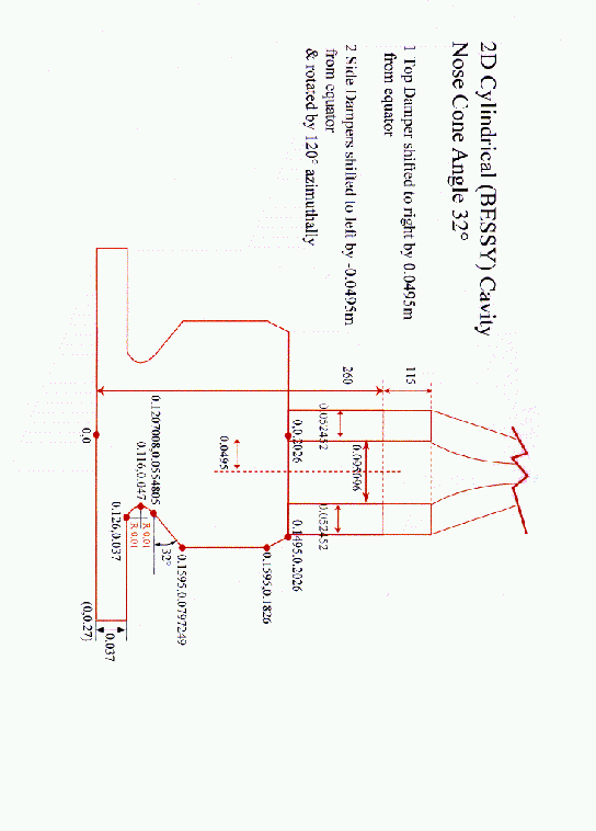
We got detailed technical data1 of the proposed BESSY cavity.
The technical data are transformed step by step into an inputfile for gd1. Every step is explained in detail. Numerous hints are given, how one effectively models the geometry.
 |
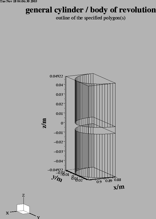
In the first step we model the cavity and the beam-pipes. We do this by specifying a polygonal description of the boundary in the r-z-plane. The inputfile that describes the boundary is:
#
# Some helpful symbols:
#
define(EL, 1) define(MAG, 2)
define(INF, 1000)
#
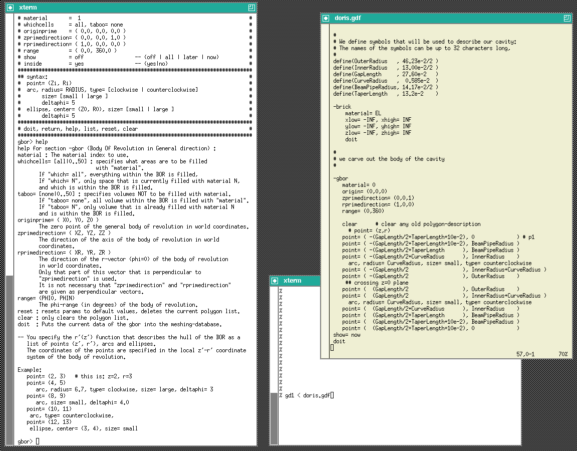
# We define symbols that will be used to describe our cavity:
# The names of the symbols can be up to 32 characters long,
#
define(OuterRadius , 46.23e-2/2 )
define(InnerRadius , 13.00e-2/2 )
define(GapLength , 27.60e-2 )
define(CurveRadius , 0.585e-2 )
define(BeamPipeRadius, 14.17e-2/2 )
define(TaperLength , 13.2e-2 )
########
#
# We fill the universe with metal
#
-brick
material= EL
xlow= -INF, xhigh= INF
ylow= -INF, yhigh= INF
zlow= -INF, zhigh= INF
doit
#
# we carve out the body of the cavity
#
-gbor
material= 0
origin= (0,0,0)
range= (0,360)
clear
#
# the following polygon describes the upper part of the cavity:
#
point= ( -1e-6, 0) # (z,r)
point= ( 0.1+0.27, 0)
point= ( 0.1+0.27, 0.037 )
point= ( 0.126, 0.037)
arc, radius= 0.01, size= small, type= clockwise
point= ( 0.116, 0.047)
arc,
point= ( 0.1207008, 0.0554805 )
point= ( 0.1595, 0.0797249 )
point= ( 0.1595, 0.1836 )
point= ( 0.1495, 0.2027 ) # 0.2027 am 7.ten November 2003
point= ( 0, 0.2027 )
point= ( -1e-6, 0 )
#
# specify the r- and z-direction of the BOR,
# model the upper part.
#
rprime= ( 1, 0, 0 )
zprime= ( 0, 0, 1 ) # Upper part of the cavity
show= later
doit
#
# re-specify the z-direction,
# model the lower part.
#
zprime= ( 0, 0, -1 ) # lower part of the cavity
show= all
doit
-volumeplot
doit
This inputfile can be found as "/usr/local/gd1/Tutorial-Bessy/bessy00.gdf".
When we feed this file into gd1 via the command
"gd1 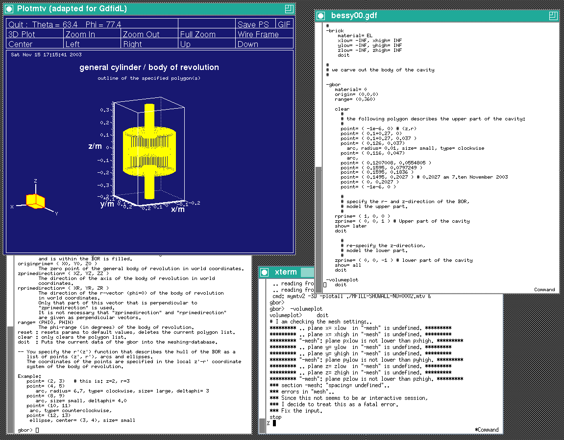 |
gd1 does not what we want, we do not get a "volumeplot", although we requested one. But gd1 gives us a hint what we made wrong:
 gbor>  -volumeplot
 volumeplot>     doit
 # I am checking the mesh settings..
 ********* .. plane x= xlow  in "-mesh" is undefined. *********
 ********* .. plane x= xhigh in "-mesh" is undefined. *********
 ********* "-mesh": plane pxlow is not lower than pxhigh. *********
 ********* .. plane y= ylow  in "-mesh" is undefined. *********
 ********* .. plane y= yhigh in "-mesh" is undefined. *********
 ********* "-mesh": plane pylow is not lower than pyhigh. *********
 ********* .. plane z= zlow  in "-mesh" is undefined. *********
 ********* .. plane z= zhigh in "-mesh" is undefined. *********
 ********* "-mesh": plane pzlow is not lower than pzhigh. *********
 *** section -mesh: "spacing= undefined"..
 *** errors in "mesh"..
 *** Since this not seems to be an interactive session,
 *** I decide to treat this as a fatal error.
 *** Fix the input.
 stop
When we say "doit" in the section "-volumeplot", gd1 tries to generate the mesh. But in order to generate the mesh, gd1 needs to know
To give gd1 the needed information, we change our inputfile. We insert the following lines somewhere before "-volumeplot":
 ###
 ### We define the borders of the computational volume,
 ### and we define the default mesh-spacing.
 ###
 -mesh
     spacing= InnerRadius/15
     pxlow= -1.1*OuterRadius, pxhigh= 1.1*OuterRadius
     pylow= -1.1*OuterRadius, pyhigh= 1.1*OuterRadius
     pzlow = -(GapLength/2+TaperLength+9e-2)
     pzhigh= +(GapLength/2+TaperLength+9e-2)
The so edited inputfile can be found as
"/usr/local/gd1/Tutorial-Bessy/bessy01.gdf".
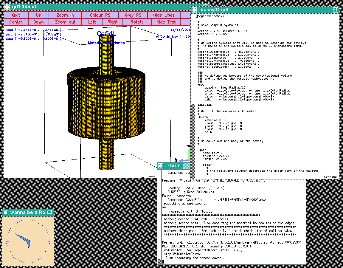
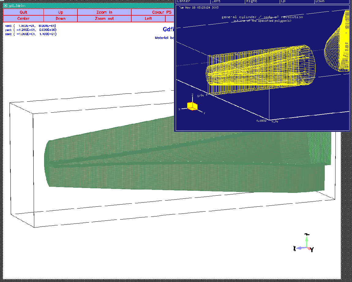
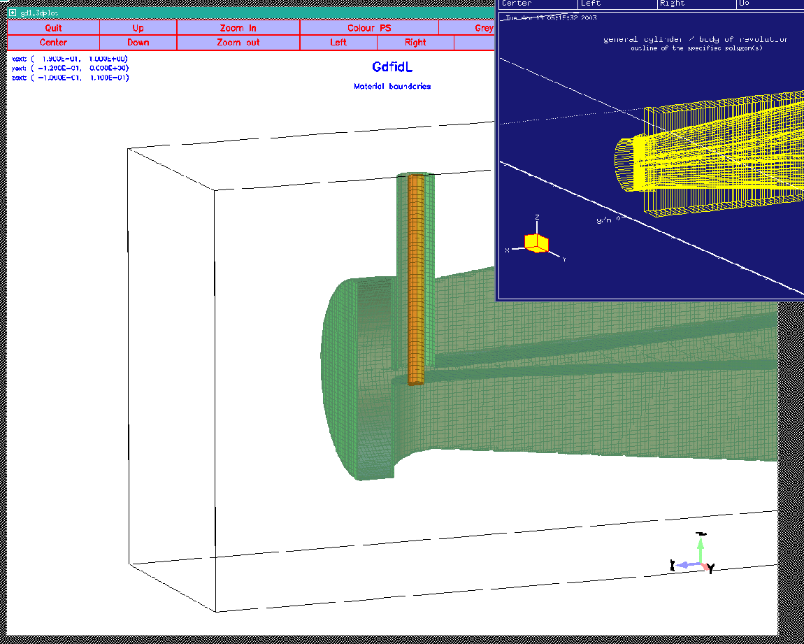
When we feed gd1 with this inputfile (gd1 ![]() bessy01.gdf)
we get a screen similiar to the one shown in figure 1.4
bessy01.gdf)
we get a screen similiar to the one shown in figure 1.4
 |
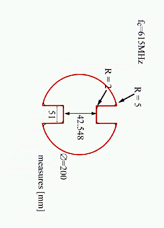
The hollow waveguide section is a ridged waveguide where the cross section varies continously. The waveguide is designed such, that at every cross section the cutoff frequency of the fundamental mode is the same.
The waveguides a general cylinders, where the cross section of the cylinders is some polygon. gd1 can model this directly. We edit our inputfile so that it contains:
 define(GuideR0, 200e-3/2)
 define(GuideGap, 42.548e-3)
 define(WW, 51e-3)
 define(RR2, 2e-3)
 define(RR5, 5e-3)

 -ggcylinder
    material= 0
    range= ( 0, 100e-3 )

 define(AA, WW/2+RR5)
 define(BB, ((GuideR0-RR5)**2 - AA**2)**0.5)
 define(THETA, atan2(BB, AA))

    clear

       # +x, +y
       point= ( GuideR0, 0 ) # x', y'
          arc, radius= GuideR0, size= small, type= counterclockwise, deltaphi= 5
       point= ( GuideR0*cos(THETA), GuideR0*sin(THETA) )
          arc, radius= RR5, size= small, type= counterclockwise, , deltaphi= 15
       point= (  WW/2   , BB )
       point= (  WW/2   , GuideGap/2+ RR2 )
          arc, radius= RR2, size= small, type= clockwise
       point= (  WW/2-RR2 , GuideGap/2 )

       # -x, +y
       point= ( -(WW/2-RR2), GuideGap/2 )
          arc, radius= RR2, size= small, type= clockwise
       point= ( -WW/2   , GuideGap/2+ RR2 )
       point= ( -WW/2   , BB )
          arc, radius= RR5, size= small, type= counterclockwise, , deltaphi= 15
       point= ( -GuideR0*cos(THETA), GuideR0*sin(THETA) )
          arc, radius= GuideR0, size= small, type= counterclockwise, deltaphi= 5
       point= ( -GuideR0, 0 ) # x', y'

       # -x, -y
       point= ( -GuideR0, 0 ) # x', y'
          arc, radius= GuideR0, size= small, type= counterclockwise, deltaphi= 5
       point= ( -GuideR0*cos(THETA), -GuideR0*sin(THETA) )
          arc, radius= RR5, size= small, type= counterclockwise, , deltaphi= 15
       point= (  -WW/2   , -BB )
       point= (  -WW/2   , -(GuideGap/2+ RR2) )
          arc, radius= RR2, size= small, type= clockwise
       point= (  -(WW/2-RR2), -GuideGap/2 )

       # +x, -y
       point= (  (WW/2-RR2), -GuideGap/2 )
          arc, radius= RR2, size= small, type= clockwise
       point= (  WW/2   , -(GuideGap/2+ RR2) )
       point= (  WW/2   , -BB )
          arc, radius= RR5, size= small, type= counterclockwise, , deltaphi= 15
       point= (  GuideR0*cos(THETA), -GuideR0*sin(THETA) )
          arc, radius= GuideR0, size= small, type= counterclockwise, deltaphi= 5
       point= (  GuideR0, 0 ) # x', y'

   show= all
   doit
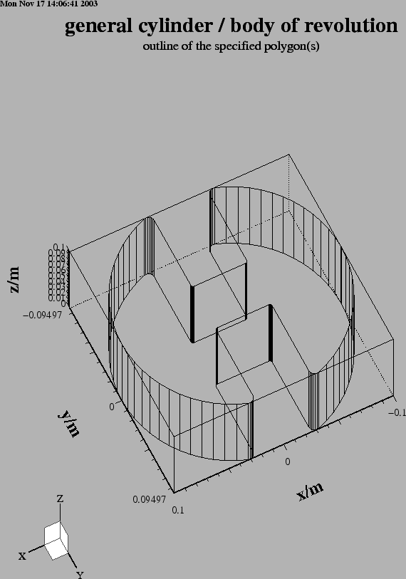
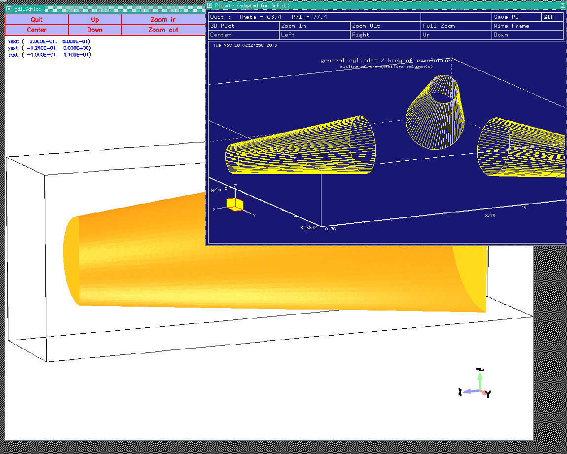
The figure 1.6 shows an outline of the waveguide that
this decribes.
This waveguide has its axis gowing in z-direction.
Our waveguides shall have their axis lying in the x-y-plane,
with an angle of 0, 120 and 240 degrees.
In order to have the axis of our waveguide direct in the proper direction, we
change the values of xprimedirection, yprimedirection.
These two vectors define the local x', y' coordinate-system, in which
the foorprint of the general cylinder is described.
We edit our inputfile:
 -ggcylinder
    material= 0
    range= ( 0, 100e-3 )

 define(PHI, 120*@pi/180 )
    xprimedirection= ( cos(PHI-@pi/2), sin(PHI-@pi/2), 0 )
    yprimedirection= ( 0, 0, 1 )
The resulting outline is shown in figure 1.7.
macro.
Anywhere in an inputfile we can define macros.
A macro is enclosed between two lines: The first line contains the keyword
macro followed by the name of the macro.
All lines until a line with only the keyword endmacro are considered
the body of the macro.
When gd1 or gd1.pp find such a macro, they read it and store the body of the
macro in an internal buffer.
Example
   #
   # This defines a macro with name 'foo'
   #
   macro foo
      echo I am foo, my first argument is @arg1
      echo The total number of arguments supplied is @nargs
   endmacro
When gd1 or gd1.pp find a call of the macro, the number of the supplied
arguments is assigned to the variable @nargs, and the variables
@arg1, @arg2, .. are assigned the values of the supplied parameters
of the call.
The values of the arguments are strings. Of course it is possible
to have a string eg. '1e-4' which happens to be interpreted in the
right context as a real number.
   #
   # this calls 'foo' with the arguments 'hi', 'there'
   #
   call foo(hi, there)
Macro calls may be nested. The body of a macro may call another macro.
 macro Waveguide
    define(Angle, @arg1)     # First argument of the macro
    define(ZPOSITION, @arg2) # Second argument

    define(GuideR0, 200e-3/2)
    define(GuideGap, 42.548e-3)
    define(WW, 51e-3)
    define(RR2, 2e-3)
    define(RR5, 5e-3)

 -ggcylinder
    material= 0
    range= ( 0, 100e-3 )

 define(PHI, Angle*@pi/180 )
    xprimedirection= ( cos(PHI-@pi/2), sin(PHI-@pi/2), 0 )
    yprimedirection= ( 0, 0, 1 )
    origin= ( 100*cos(PHI), 100*sin(PHI), ZPOSITION )

 define(AA, WW/2+RR5)
 define(BB, ((GuideR0-RR5)**2 - AA**2)**0.5)
 define(THETA, atan2(BB, AA))

    clear

       # +x, +y
       point= ( GuideR0, 0 ) # x', y'
          arc, radius= GuideR0, size= small, type= counterclockwise, deltaphi= 5
       point= ( GuideR0*cos(THETA), GuideR0*sin(THETA) )
          arc, radius= RR5, size= small, type= counterclockwise, , deltaphi= 15
       point= (  WW/2   , BB )
       point= (  WW/2   , GuideGap/2+ RR2 )
          arc, radius= RR2, size= small, type= clockwise
       point= (  WW/2-RR2 , GuideGap/2 )

       # -x, +y
       point= ( -(WW/2-RR2), GuideGap/2 )
          arc, radius= RR2, size= small, type= clockwise
       point= ( -WW/2   , GuideGap/2+ RR2 )
       point= ( -WW/2   , BB )
          arc, radius= RR5, size= small, type= counterclockwise, , deltaphi= 15
       point= ( -GuideR0*cos(THETA), GuideR0*sin(THETA) )
          arc, radius= GuideR0, size= small, type= counterclockwise, deltaphi= 5
       point= ( -GuideR0, 0 ) # x', y'

       # -x, -y
       point= ( -GuideR0, 0 ) # x', y'
          arc, radius= GuideR0, size= small, type= counterclockwise, deltaphi= 5
       point= ( -GuideR0*cos(THETA), -GuideR0*sin(THETA) )
          arc, radius= RR5, size= small, type= counterclockwise, , deltaphi= 15
       point= (  -WW/2   , -BB )
       point= (  -WW/2   , -(GuideGap/2+ RR2) )
          arc, radius= RR2, size= small, type= clockwise
       point= (  -(WW/2-RR2), -GuideGap/2 )

       # +x, -y
       point= (  (WW/2-RR2), -GuideGap/2 )
          arc, radius= RR2, size= small, type= clockwise
       point= (  WW/2   , -(GuideGap/2+ RR2) )
       point= (  WW/2   , -BB )
          arc, radius= RR5, size= small, type= counterclockwise, , deltaphi= 15
       point= (  GuideR0*cos(THETA), -GuideR0*sin(THETA) )
          arc, radius= GuideR0, size= small, type= counterclockwise, deltaphi= 5
       point= (  GuideR0, 0 ) # x', y'

   show= all
   doit
 endmacro
To be able to model the complicated second part, we model the waveguide in two steps. In the first step, we fill a volume with vacuum. This volume models the waveguide without the ridge, ie it is simply a circulare waveguide where the radius varies linearly. In a second step, the volume of the ridge is refilled with electric conducting material.
 |
 macro Linear_Waveguide
    define(zzPHI, @arg1 *@pi/180)     # First argument of the macro
    define(ZPOSITION, @arg2)          # Second argument

    define(GuideR0, @arg4)

 -ggcylinder
    material= 0
    range= ( @arg3, @arg5 )

    xprimedirection= ( cos(zzPHI+@pi/2), sin(zzPHI+@pi/2), 0 )
    yprimedirection= ( 0, 0, 1 )
    origin= ( 0, 0, ZPOSITION )

 xslope= (@arg6/@arg4-1)/(@arg5-@arg3)
 yslope= (@arg6/@arg4-1)/(@arg5-@arg3)

    clear

       point= ( GuideR0, 0 ) # x', y'
          arc, radius= GuideR0, size= small, type= counterclockwise, deltaphi= 5
       point= ( 0, GuideR0 )
          arc,
       point= ( -GuideR0, 0 )
          arc,
       point= ( 0, -GuideR0 )
          arc,
       point= ( GuideR0, 0 )

   show= @arg7 # now|later|all
   doit
 endmacro

 if (0) then
    #
    # for example, call the macro three times:
    #
    do Phi= 0, 240, 120
       if (Phi == 240) then
          sdefine(SHOW, all)
       else
          sdefine(SHOW, later)
       endif
    call Linear_Waveguide(Phi, \   # angle
                          10e-3, \ # z-position
                          260e-3, \           # starting position of the ggcylinder
                          100e-3, \           # start value outer radius
                          (260e-3+500e-3), \  # end position of the ggcylinder
                          50e-3, \            # endvalue of the outer radius
                          SHOW )
    enddo
 endif
 |
 macro Linear_Ridge
    define(zzPHI, @arg1 *@pi/180)     # First argument of the macro
    define(ZPOSITION, @arg2)          # Second argument
    define(GuideGap, 2*(@arg4) )      # @arg4 : Half starting gap

    define(WW, 51e-3)
    define(RR2, 2e-3)
    define(RR5, 5e-3)

 -ggcylinder
    range= ( @arg3, @arg5 )

    xprimedirection= ( cos(zzPHI+@pi/2), sin(zzPHI+@pi/2), 0 )
    yprimedirection= ( 0, 0, 1 )
    origin= ( 0, 0, ZPOSITION )

    #
    # We first refill a larger part with
    # electric conducting material.
    #
    clear
       point= ( -WW/2, -100e-3 ) # x', y'
       point= (  WW/2, -100e-3 )
       point= (  WW/2,  100e-3 )
       point= ( -WW/2,  100e-3 )
    material= 3
    show= later
    xslope= 0, yslope= 0
    doit


    #
    # We now carve out the vacuum part
    #
    material= 0
 xslope= 0
 yslope= (@arg6/@arg4-1)/(@arg5-@arg3)

 define(AA, WW/2+RR5)
 define(BB, ((GuideR0-RR5)**2 - AA**2)**0.5)
 define(THETA, atan2(BB, AA))

    clear

       # +x, +y
       point= (  WW/2   , GuideGap/2+ RR2 )
          arc, radius= RR2, size= small, type= clockwise
       point= (  WW/2-RR2 , GuideGap/2 )

       # -x, +y
       point= ( -(WW/2-RR2), GuideGap/2 )
          arc, radius= RR2, size= small, type= clockwise
       point= ( -WW/2   , GuideGap/2+ RR2 )

       # -x, -y
       point= (  -WW/2   , -(GuideGap/2+ RR2) )
          arc, radius= RR2, size= small, type= clockwise
       point= (  -(WW/2-RR2), -GuideGap/2 )

       # +x, -y
       point= (  (WW/2-RR2), -GuideGap/2 )
          arc, radius= RR2, size= small, type= clockwise
       point= (  WW/2   , -(GuideGap/2+ RR2) )

   show= @arg7 # now|later|all
   doit
 endmacro

 #
 # Call the macro for example like this:
 #
 if (0) then
    call Linear_Ridge(0, \   # angle
                      10e-3, \ # z-position
                      260e-3, \           # starting position of the ggcylinder
                      43e-3, \           # start value half gap
                      (260e-3+500e-3), \  # end position of the ggcylinder
                      9e-3, \            # endvalue of half gap
                      all )
 endif
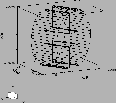
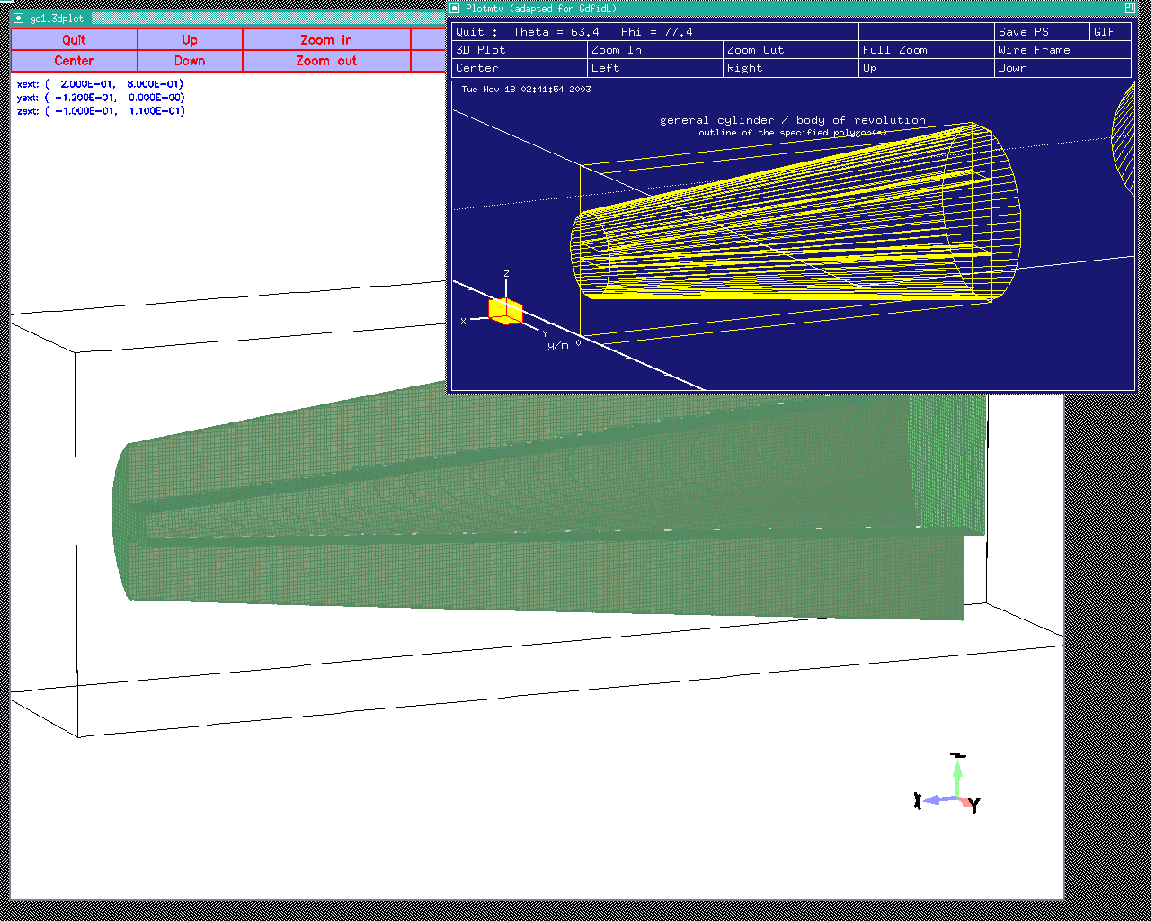
When we call the macro after the linear varying waveguide has been modeled,
we get a plot similiar to the one shown in figure 2.3.
The used inputfile is:
 -brick
    material= 3
    volume= ( -INF,INF, -INF,INF, -INF,INF )
    doit

 include( macro-Linear_Waveguide.gdf )
 include( macro-Linear_Ridge.gdf )

 #
 # Call the macros three times:
 #
 do Phi= 0, 240, 120
    if (Phi == 240) then
       sdefine(SHOW, all)
    else
       sdefine(SHOW, later)
    endif
    call Linear_Waveguide(Phi, \   # angle
                          10e-3, \ # z-position
                          260e-3, \           # starting position of the ggcylinder
                          100e-3, \           # start value outer radius
                          (260e-3+500e-3), \  # end position of the ggcylinder
                          50e-3, \            # endvalue of the outer radius
                          later )


    call Linear_Ridge(Phi, \   # angle
                      10e-3, \ # z-position
                      260e-3, \           # starting position of the ggcylinder
                      43e-3, \           # start value half gap
                      (260e-3+500e-3), \  # end position of the ggcylinder
                      9e-3, \            # endvalue of half gap
                      SHOW )
 enddo


 -mesh
    perfectmesh= yes
    spacing= 2e-3
    pxlow= 0.2, pxhigh= 0.8
    pylow= -0.12, pyhigh= 0
    pzlow= -0.1, pzhigh= 0.11

 -volumeplot
     doit
 |
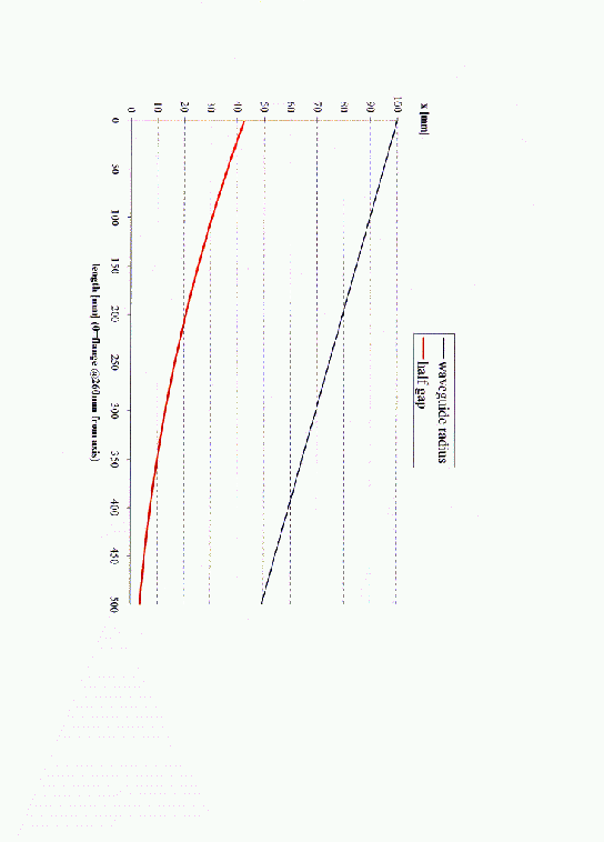
Since the real ridgevaries nonlinearly, we now have to call the macro many times with the proper start and end values. The wanted gap-widths as a function position can be taken from the dataset provided by Dr Marhauser:
1. Waveguide Position
2. Waveguide Radius
3. Half Gap-distance
4. Distance measured from Cavity-adapter
5. Distance measured from Cavity-center
0       100             42.548  115     375
10      98.98448        41.2529 125     385
20      97.96896        39.9786 135     395
30      96.95344        38.7253 145     405
40      95.93792        37.4932 155     415
50      94.9224         36.2822 165     425
60      93.90688        35.0925 175     435
70      92.89136        33.9242 185     445
80      91.87584        32.7772 195     455
90      90.86032        31.6517 205     465
100     89.8448         30.5478 215     475
110     88.82928        29.4654 225     485
120     87.81376        28.4046 235     495
130     86.79824        27.3812 245     505
140     85.78272        26.3479 255     515
150     84.76720        25.3521 265     525
160     83.75168        24.378  275     535
170     82.73616        23.4255 285     545
180     81.72064        22.4947 295     555
190     80.70512        21.5856 305     565
200     79.68960        20.6981 315     575
210     78.67408        19.8322 325     585
220     77.65856        18.9879 335     595
230     76.64304        18.165  345     605
240     75.62752        17.3635 355     615
250     74.61200        16.5834 365     625
260     73.59648        15.8246 375     635
270     72.58096        15.0868 385     645
280     71.56544        14.3701 395     655
290     70.54992        13.6743 405     665
300     69.53440        12.9992 415     675
310     68.51888        12.3448 425     685
320     67.50336        11.7107 435     695
330     66.48784        11.0969 445     705
340     65.47232        10.5031 455     715
350     64.45680        9.92909 465     725
360     63.44128        9.3747  475     735
370     62.42576        8.83965 485     745
380     61.41024        8.32367 495     755
390     60.39472        7.82648 505     765
400     59.37920        7.3478  515     775
410     58.36368        6.88729 525     785
420     57.34816        6.44464 535     795
430     56.33264        6.01949 545     805
440     55.31712        5.61147 555     815
450     54.30160        5.22019 565     825
460     53.28608        4.84526 575     835
470     52.27056        4.48623 585     845
480     51.25504        4.14267 595     855
490     50.23952        3.8141  605     865
500     49.22400        3.5000  615     875
We can generate the needed calls to our function via a short program tha reads this dataset and then writes the appropriate file:
 ! This is a small Fortran program which generates
 ! the appropriate calls.

    DO i= 1, 5
       READ (*,*) ! Skip the first five lines
    ENDDO

    DO
       READ (*,*) WPos, WRadius, HGap, DistAdapt, DistanceCenter
       WRITE (*,50) DistanceCenter*1e-3, HGap*1e-3
       WRITE (*,60) DistanceCenter*1e-3
       WRITE (*,70)                  HGap*1e-3
    ENDDO

 50 FORMAT(' call Linear_Ridge(Phi, ZPOS,', &
            G17.7,', ', G17.7,', POS_OLD, G_OLD, later )')
 60 FORMAT(' ')
 70 FORMAT(' ')

    END
The inputfile with the automaticalls generated calls:
 -brick
    material= 3
    volume= ( -INF,INF, -INF,INF, -INF,INF )
    doit

 include( macro-Linear_Waveguide.gdf )
 include( macro-Linear_Ridge.gdf )

 #
 # Call the macros three times:
 #
 do Phi= 0, 240, 120
    if (Phi == 240) then
       sdefine(SHOW, all)
    else
       sdefine(SHOW, later)
    endif
 define(ZPOS, 10e-3)

    #
    # constant radius section:
    #
    call Linear_Waveguide(Phi, \   # angle
                          ZPOS, \ # z-position
                          200e-3, \           # starting position of the ggcylinder
                          100e-3, \           # start value outer radius
                          375e-3, \  # end position of the ggcylinder
                          100e-3, \            # endvalue of the outer radius
                          later )

    #
    # linear varying section:
    #
    call Linear_Waveguide(Phi, \   # angle
                          ZPOS, \ # z-position
                          375e-3, \           # starting position of the ggcylinder
                          100e-3, \           # start value outer radius
                          (375e-3+500e-3), \  # end position of the ggcylinder
                          50e-3, \            # endvalue of the outer radius
                          later )


 define(POS_OLD,    0.200000     ) # inserted by hand
 define(G_OLD,    0.4254800E-01 )  # inserted by hand
 #
 # The automatically generated part of the inputfile:
 #
 call Linear_Ridge(Phi, ZPOS,    0.2600000    ,     0.4254800E-01, POS_OLD, G_OLD, later )
 define(POS_OLD,    0.2600000     )
 define(G_OLD,    0.4254800E-01 )
 call Linear_Ridge(Phi, ZPOS,    0.2700000    ,     0.4125290E-01, POS_OLD, G_OLD, later )
 define(POS_OLD,    0.2700000     )
 define(G_OLD,    0.4125290E-01 )
 call Linear_Ridge(Phi, ZPOS,    0.2800000    ,     0.3997860E-01, POS_OLD, G_OLD, later )
 define(POS_OLD,    0.2800000     )
 define(G_OLD,    0.3997860E-01 )
 call Linear_Ridge(Phi, ZPOS,    0.2900000    ,     0.3872530E-01, POS_OLD, G_OLD, later )
 define(POS_OLD,    0.2900000     )
 define(G_OLD,    0.3872530E-01 )
 call Linear_Ridge(Phi, ZPOS,    0.3000000    ,     0.3749320E-01, POS_OLD, G_OLD, later )
 define(POS_OLD,    0.3000000     )
 define(G_OLD,    0.3749320E-01 )
 call Linear_Ridge(Phi, ZPOS,    0.3100000    ,     0.3628220E-01, POS_OLD, G_OLD, later )
 define(POS_OLD,    0.3100000     )
 define(G_OLD,    0.3628220E-01 )
 call Linear_Ridge(Phi, ZPOS,    0.3200000    ,     0.3509250E-01, POS_OLD, G_OLD, later )
 define(POS_OLD,    0.3200000     )
 define(G_OLD,    0.3509250E-01 )
 call Linear_Ridge(Phi, ZPOS,    0.3300000    ,     0.3392420E-01, POS_OLD, G_OLD, later )
 define(POS_OLD,    0.3300000     )
 define(G_OLD,    0.3392420E-01 )
 call Linear_Ridge(Phi, ZPOS,    0.3400000    ,     0.3277720E-01, POS_OLD, G_OLD, later )
 define(POS_OLD,    0.3400000     )
 define(G_OLD,    0.3277720E-01 )
 call Linear_Ridge(Phi, ZPOS,    0.3500000    ,     0.3165170E-01, POS_OLD, G_OLD, later )
 define(POS_OLD,    0.3500000     )
 define(G_OLD,    0.3165170E-01 )
 call Linear_Ridge(Phi, ZPOS,    0.3600000    ,     0.3054780E-01, POS_OLD, G_OLD, later )
 define(POS_OLD,    0.3600000     )
 define(G_OLD,    0.3054780E-01 )
 call Linear_Ridge(Phi, ZPOS,    0.3700000    ,     0.2946540E-01, POS_OLD, G_OLD, later )
 define(POS_OLD,    0.3700000     )
 define(G_OLD,    0.2946540E-01 )
 call Linear_Ridge(Phi, ZPOS,    0.3800000    ,     0.2840460E-01, POS_OLD, G_OLD, later )
 define(POS_OLD,    0.3800000     )
 define(G_OLD,    0.2840460E-01 )
 call Linear_Ridge(Phi, ZPOS,    0.3900000    ,     0.2738120E-01, POS_OLD, G_OLD, later )
 define(POS_OLD,    0.3900000     )
 define(G_OLD,    0.2738120E-01 )
 call Linear_Ridge(Phi, ZPOS,    0.4000000    ,     0.2634790E-01, POS_OLD, G_OLD, later )
 define(POS_OLD,    0.4000000     )
 define(G_OLD,    0.2634790E-01 )
 call Linear_Ridge(Phi, ZPOS,    0.4100000    ,     0.2535210E-01, POS_OLD, G_OLD, later )
 define(POS_OLD,    0.4100000     )
 define(G_OLD,    0.2535210E-01 )
 call Linear_Ridge(Phi, ZPOS,    0.4200000    ,     0.2437800E-01, POS_OLD, G_OLD, later )
 define(POS_OLD,    0.4200000     )
 define(G_OLD,    0.2437800E-01 )
 call Linear_Ridge(Phi, ZPOS,    0.4300000    ,     0.2342550E-01, POS_OLD, G_OLD, later )
 define(POS_OLD,    0.4300000     )
 define(G_OLD,    0.2342550E-01 )
 call Linear_Ridge(Phi, ZPOS,    0.4400000    ,     0.2249470E-01, POS_OLD, G_OLD, later )
 define(POS_OLD,    0.4400000     )
 define(G_OLD,    0.2249470E-01 )
 call Linear_Ridge(Phi, ZPOS,    0.4500000    ,     0.2158560E-01, POS_OLD, G_OLD, later )
 define(POS_OLD,    0.4500000     )
 define(G_OLD,    0.2158560E-01 )
 call Linear_Ridge(Phi, ZPOS,    0.4600000    ,     0.2069810E-01, POS_OLD, G_OLD, later )
 define(POS_OLD,    0.4600000     )
 define(G_OLD,    0.2069810E-01 )
 call Linear_Ridge(Phi, ZPOS,    0.4700000    ,     0.1983220E-01, POS_OLD, G_OLD, later )
 define(POS_OLD,    0.4700000     )
 define(G_OLD,    0.1983220E-01 )
 call Linear_Ridge(Phi, ZPOS,    0.4800000    ,     0.1898790E-01, POS_OLD, G_OLD, later )
 define(POS_OLD,    0.4800000     )
 define(G_OLD,    0.1898790E-01 )
 call Linear_Ridge(Phi, ZPOS,    0.4900000    ,     0.1816500E-01, POS_OLD, G_OLD, later )
 define(POS_OLD,    0.4900000     )
 define(G_OLD,    0.1816500E-01 )
 call Linear_Ridge(Phi, ZPOS,    0.5000000    ,     0.1736350E-01, POS_OLD, G_OLD, later )
 define(POS_OLD,    0.5000000     )
 define(G_OLD,    0.1736350E-01 )
 call Linear_Ridge(Phi, ZPOS,    0.5100001    ,     0.1658340E-01, POS_OLD, G_OLD, later )
 define(POS_OLD,    0.5100001     )
 define(G_OLD,    0.1658340E-01 )
 call Linear_Ridge(Phi, ZPOS,    0.5200000    ,     0.1582460E-01, POS_OLD, G_OLD, later )
 define(POS_OLD,    0.5200000     )
 define(G_OLD,    0.1582460E-01 )
 call Linear_Ridge(Phi, ZPOS,    0.5300000    ,     0.1508680E-01, POS_OLD, G_OLD, later )
 define(POS_OLD,    0.5300000     )
 define(G_OLD,    0.1508680E-01 )
 call Linear_Ridge(Phi, ZPOS,    0.5400000    ,     0.1437010E-01, POS_OLD, G_OLD, later )
 define(POS_OLD,    0.5400000     )
 define(G_OLD,    0.1437010E-01 )
 call Linear_Ridge(Phi, ZPOS,    0.5500000    ,     0.1367430E-01, POS_OLD, G_OLD, later )
 define(POS_OLD,    0.5500000     )
 define(G_OLD,    0.1367430E-01 )
 call Linear_Ridge(Phi, ZPOS,    0.5600000    ,     0.1299920E-01, POS_OLD, G_OLD, later )
 define(POS_OLD,    0.5600000     )
 define(G_OLD,    0.1299920E-01 )
 call Linear_Ridge(Phi, ZPOS,    0.5700001    ,     0.1234480E-01, POS_OLD, G_OLD, later )
 define(POS_OLD,    0.5700001     )
 define(G_OLD,    0.1234480E-01 )
 call Linear_Ridge(Phi, ZPOS,    0.5800000    ,     0.1171070E-01, POS_OLD, G_OLD, later )
 define(POS_OLD,    0.5800000     )
 define(G_OLD,    0.1171070E-01 )
 call Linear_Ridge(Phi, ZPOS,    0.5900000    ,     0.1109690E-01, POS_OLD, G_OLD, later )
 define(POS_OLD,    0.5900000     )
 define(G_OLD,    0.1109690E-01 )
 call Linear_Ridge(Phi, ZPOS,    0.6000000    ,     0.1050310E-01, POS_OLD, G_OLD, later )
 define(POS_OLD,    0.6000000     )
 define(G_OLD,    0.1050310E-01 )
 call Linear_Ridge(Phi, ZPOS,    0.6100000    ,     0.9929090E-02, POS_OLD, G_OLD, later )
 define(POS_OLD,    0.6100000     )
 define(G_OLD,    0.9929090E-02 )
 call Linear_Ridge(Phi, ZPOS,    0.6200000    ,     0.9374700E-02, POS_OLD, G_OLD, later )
 define(POS_OLD,    0.6200000     )
 define(G_OLD,    0.9374700E-02 )
 call Linear_Ridge(Phi, ZPOS,    0.6300001    ,     0.8839651E-02, POS_OLD, G_OLD, later )
 define(POS_OLD,    0.6300001     )
 define(G_OLD,    0.8839651E-02 )
 call Linear_Ridge(Phi, ZPOS,    0.6400000    ,     0.8323670E-02, POS_OLD, G_OLD, later )
 define(POS_OLD,    0.6400000     )
 define(G_OLD,    0.8323670E-02 )
 call Linear_Ridge(Phi, ZPOS,    0.6500000    ,     0.7826480E-02, POS_OLD, G_OLD, later )
 define(POS_OLD,    0.6500000     )
 define(G_OLD,    0.7826480E-02 )
 call Linear_Ridge(Phi, ZPOS,    0.6600000    ,     0.7347800E-02, POS_OLD, G_OLD, later )
 define(POS_OLD,    0.6600000     )
 define(G_OLD,    0.7347800E-02 )
 call Linear_Ridge(Phi, ZPOS,    0.6700000    ,     0.6887290E-02, POS_OLD, G_OLD, later )
 define(POS_OLD,    0.6700000     )
 define(G_OLD,    0.6887290E-02 )
 call Linear_Ridge(Phi, ZPOS,    0.6800000    ,     0.6444640E-02, POS_OLD, G_OLD, later )
 define(POS_OLD,    0.6800000     )
 define(G_OLD,    0.6444640E-02 )
 call Linear_Ridge(Phi, ZPOS,    0.6900001    ,     0.6019490E-02, POS_OLD, G_OLD, later )
 define(POS_OLD,    0.6900001     )
 define(G_OLD,    0.6019490E-02 )
 call Linear_Ridge(Phi, ZPOS,    0.7000000    ,     0.5611470E-02, POS_OLD, G_OLD, later )
 define(POS_OLD,    0.7000000     )
 define(G_OLD,    0.5611470E-02 )
 call Linear_Ridge(Phi, ZPOS,    0.7100000    ,     0.5220190E-02, POS_OLD, G_OLD, later )
 define(POS_OLD,    0.7100000     )
 define(G_OLD,    0.5220190E-02 )
 call Linear_Ridge(Phi, ZPOS,    0.7200000    ,     0.4845260E-02, POS_OLD, G_OLD, later )
 define(POS_OLD,    0.7200000     )
 define(G_OLD,    0.4845260E-02 )
 call Linear_Ridge(Phi, ZPOS,    0.7300000    ,     0.4486230E-02, POS_OLD, G_OLD, later )
 define(POS_OLD,    0.7300000     )
 define(G_OLD,    0.4486230E-02 )
 call Linear_Ridge(Phi, ZPOS,    0.7400000    ,     0.4142670E-02, POS_OLD, G_OLD, later )
 define(POS_OLD,    0.7400000     )
 define(G_OLD,    0.4142670E-02 )
 call Linear_Ridge(Phi, ZPOS,    0.7500001    ,     0.3814100E-02, POS_OLD, G_OLD, later )
 define(POS_OLD,    0.7500001     )
 define(G_OLD,    0.3814100E-02 )
 call Linear_Ridge(Phi, ZPOS,    0.7600001    ,     0.3500000E-02, POS_OLD, G_OLD, SHOW )
 define(POS_OLD,    0.7600001     )
 define(G_OLD,    0.3500000E-02 )

 enddo


 -mesh
    perfectmesh= yes
    spacing= 2e-3
    pxlow= 0.19, pxhigh= 0.8
    pylow= -0.12, pyhigh= 0
    pzlow= -0.1, pzhigh= 0.11

 -volumeplot
     doit
 |
 macro transformer
    define(zzPHI, (@arg1)*@pi/180 )
    define(ZOFF, @arg2)

    define(RALT, 50e-3) # The last radius
    -ggcyl
         material= 1
         xprime= ( cos(zzPHI      ), sin(zzPHI      ), 0 )
         yprime= ( cos(zzPHI+@pi/2), sin(zzPHI+@pi/2), 0 )
         xslope= 0, yslope= 0
 define(RR, 906.0e-3 - 31e-3)
 echo *** r-Position of tip of ellipse: eval(RR+31e-3) ( should be 906.0e-3 )
         origin= ( RR*cos(zzPHI), RR*sin(zzPHI), ZOFF )
         clear
            point= ( 0, -51e-3/2 )
               ellipse, center= ( 0, 0 ), size= small
            point= ( 31e-3, 0 )
               ellipse
            point= ( 0,  51e-3/2 )
         range= ( 3.5e-3, RALT )
    show= later
         doit
         range= ( -RALT, -3.5e-3 )
    show= @arg3
         doit

 endmacro

 if (0) then
    #
    # Call this macro eg like this:
    #
    call transformer(0, 0, later )
 endif
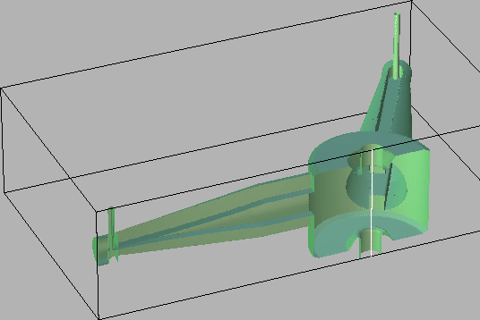
The coaxial waveguides are easily described as circular cylinders. In the first step, a circular cylinder is carved out with a radius of the outer conductor. In the second step, the volume of the inner conductor is refilled. We add these cylinders to the previous macro and get:
 macro transformer_and_coaxial
    define(zzPHI, (@arg1)*@pi/180 )
    define(ZOFF, @arg2)

    define(RALT, 50e-3) # The last radius
    -ggcyl
         material= 3
         xprime= ( cos(zzPHI      ), sin(zzPHI      ), 0 )
         yprime= ( cos(zzPHI+@pi/2), sin(zzPHI+@pi/2), 0 )
         xslope= 0, yslope= 0
 define(RR, 906.0e-3 - 31e-3)
 echo *** r-Position of tip of ellipse: eval(RR+31e-3) ( should be 906.0e-3 )
         origin= ( RR*cos(zzPHI), RR*sin(zzPHI), ZOFF )
         clear
            point= ( 0, -51e-3/2 )
               ellipse, center= ( 0, 0 ), size= small
            point= ( 31e-3, 0 )
               ellipse
            point= ( 0,  51e-3/2 )
         range= ( 3.5e-3, RALT )
    show= later
         doit
         range= ( -RALT, -3.5e-3 )
    show= @arg3
         doit

    #
    # The coaxial line:
    #
    ### r-Position of coaxial lines:
    define(RR, 894.2e-3-19.2e-3)

    define(XOFF, (RR+19.2e-3)*cos(zzPHI) )
    define(YOFF, (RR+19.2e-3)*sin(zzPHI) )

    -mesh
       zfixed( 2, -3.5e-3+ZOFF, 3.5+ZOFF )
       xfixed( 3, XOFF-19.4e-3, XOFF- 8.4e-3 )
       yfixed( 3, YOFF-19.4e-3, YOFF- 8.4e-3 )
       xfixed( 3, XOFF+ 8.4e-3, XOFF+19.4e-3 )
       yfixed( 3, YOFF+ 8.4e-3, YOFF+19.4e-3 )

    -gccylinder
       length= INF
       origin= ( XOFF, YOFF, ZOFF-3.5e-3 )
       direction= ( 0, 0, 1 )
       material= 0, radius= 19.4e-3/2, doit   # Carve out radius of outer conductor

       origin= ( XOFF, YOFF, ZOFF-4.5e-3 )
       material= 4, radius=  8.4e-3/2, doit   # Refill inner conductor

 endmacro

 # call transformer_and_coaxial(Phi, Zpos, later)
 |
 -general
    outfile= /tmp/UserName/bessy-cavity
    scratch= /tmp/UserName/bessy-scratch-

    dice= yes   # If computing in parallel, use the subvolume algorithm
##    ndpw= 24    # use 24 subvolumes per CPU
    iodice= yes # store the results on the local discs of the nodes

 -material
    material= 3, type= electric
    material= 4, type= electric

 define(STPSZE, 2e-3)
 -mesh
    spacing= STPSZE

    #
    # The borders of the computational volume:
    #
 define(YLOW, -0.94)
 define(YHIGH, 0)
    pxlow= -0.6, pxhigh= 1.0
    pylow= YLOW, pyhigh= YHIGH
    pzlow= -0.2, pzhigh= 0.2

    #
    # The conditions at the borders:
    #
    cxlow= electric, cxhigh= electric
    cylow= electric, cyhigh= magnetic
    czlow= electric, czhigh= electric

 -brick
    material= 3
    volume= ( -INF,INF, -INF,INF, -INF,INF )
    doit

 include( macro-Linear_Waveguide.gdf )
 include( macro-Linear_Ridge.gdf )
 include( macro-transformer-and-coaxial.gdf )

 #
 # Call the macros three times:
 #
 do iPhi= 1, 3
    if (iPhi == 3) then
       sdefine(SHOW, all)
    else
       sdefine(SHOW, later)
    endif
    if (iPhi == 1) then
       define(ZPOS, 0.0495)
    else
       define(ZPOS, -0.0495)
    endif

 define(Phi, 0+(iPhi-1)*120)

    #
    # constant radius section of the circular part:
    #
    call Linear_Waveguide(Phi, \   # angle
                          ZPOS, \  # z-position
                          170e-3, \   # starting position of the ggcylinder
                          100e-3, \   # start value outer radius
                          375e-3, \   # end position of the ggcylinder
                          100e-3, \   # endvalue of the outer radius
                          later )

    #
    # constant section of the ridge:
    #
    call Linear_Ridge(Phi, \   # angle
                      ZPOS, \  # z-position
                      200e-3, \    # starting position of the ggcylinder
                      43e-3, \     # start value half gap
                      375e-3, \    # end position of the ggcylinder
                      9e-3, \      # endvalue of half gap
                      later )


    #
    # linear varying section:
    #
    call Linear_Waveguide(Phi, \   # angle
                          ZPOS, \ # z-position
                          375e-3, \  # starting position of the ggcylinder
                          100e-3, \  # start value outer radius
                          875e-3, \  # end position of the ggcylinder
                          50e-3, \   # endvalue of the outer radius
                          later )

    #
    # constant radius section, the part where the transformer is in
    #
    call Linear_Waveguide(Phi, \   # angle
                          ZPOS, \ # z-position
                          875e-3, \        # starting position of the ggcylinder
                          50e-3, \         # start value outer radius
                          (875e-3+65e-3), \  # end position of the ggcylinder
                          50e-3, \            # endvalue of the outer radius
                          later )


     #
     # Model the non-linear ridge via the many calls:
     #
     include( non-linear-ridge.gdf )

     #
     # Model the transformer and the coaxial line:
     #
     call transformer_and_coaxial(Phi, ZPOS, SHOW )

     #
     # tell GdfidL that the coaxial lines
     # shall be treated as ports.
     #
 define(XX, 900e-3*cos(Phi*@pi/180) )
 define(YY, 900e-3*sin(Phi*@pi/180) )
 if (YY+50e-3 >= YLOW) then
    if (YY-50e-3 <= YHIGH) then
        #
        # Only specify the port
        # if at least a part of it
        # is really within the computational volume
        #
        -fdtd
           -ports
               name= coax-phi=Phi, plane= zhigh, npml= 20, modes= 1
                  pxlow= XX-50e-3, pxhigh= XX+50e-3
                  pylow= YY-50e-3, pyhigh= YY+50e-3
               doit
    endif
 endif

 enddo # iPhi-loop

 #
 # tell GdfidL that the beam-pipes
 # shall be treated as ports.
 #
 -fdtd
    -ports
        name= beamlow, plane= zlow, npml= 40, modes= 0
           pxlow= -100e-3, pxhigh= 100e-3
           pylow= -100e-3, pyhigh= 100e-3
        doit

        name= beamhigh, plane= zhigh, npml= 40, modes= 0
           pxlow= -100e-3, pxhigh= 100e-3
           pylow= -100e-3, pyhigh= 100e-3
        doit

 #
 # Model the cavity itself:
 #
 include(Cavity.gdf)

 -volumeplot
     doit

 #
 # Specify that we want to perform a wakepotential-computation:
 #
 -fdtd
    -lcharge
       charge= 1e-12
       xposition= 0
       yposition= 0
       sigma= 5*STPSZE
       shigh= 400

 #
 # start the computation:
 #
 -fdtd
    doit
This is the end of this tutorial.