Computations with free moving charges are done by GdfidL using the Particle in Cell algorithm (PIC). The PIC computation normally consists of three steps.
 define(STPSZE, 1/100)
 -mesh
    spacing= STPSZE           # The default grid spacing

    pxlow= -1/2, pxhigh= 1/2  # The borderplanes of the computational volume
    pylow= -1/2, pyhigh= 1/2  # pylow: Plane Y LOW
    pzlow= 0, pzhigh= 1

    cxlow= electric, cxhigh= electric # Condition at x=xlow, and at x=xhigh
    cylow= electric, cyhigh= electric
    czlow= electric, czhigh= electric

 #
 # Fill the 'universe' with vacuum:
 #
 -brick
    material= 0
       xlow= -INF, xhigh= INF
       ylow= -INF, yhigh= INF
       zlow= -INF, zhigh= INF
    doit
 -fdtd
    -clouds
       #
       # We compile the executable file with the Fortran Compiler,
       #  (which is called 'fort' on this system)
       #
       system( fortran Eject-beam.f90 -o ./Eject-a.out )

       #
       # We specify that the properties of free moving charges
       # shall be described by the executable file 'Eject-a.out'
       #
       ejectioncommand=                    Eject-a.out
In addition, we have to specify the time which shall be simulated.
And we should store some fields, to analyse the fields etc.
 define(TMAX, 2/@clight)
 -fdtd
    -time
       tmin= TMAX
       tmax= TMAX

    -storefieldsat
       name= bla
          what= both   # 'what' could be 'e', 'b' or 'both'
                       # Clouds are stored anyway
          firstsaved= 0.1 / @clight
          lastsaved=    2 / @clight
          distance=   0.1 / @clight
       doit # do not forget this.
Now we can start the computation.
 #
 # Start of computation:
 #
 -fdtd
     doit
The inputfile for this cavity is empty.gdf The sourcecode for the program describing the initial conditions for the particles is Eject-beam.f90
 -general
    infile= @last
 -3da
    symbol bla_e_5
    doit
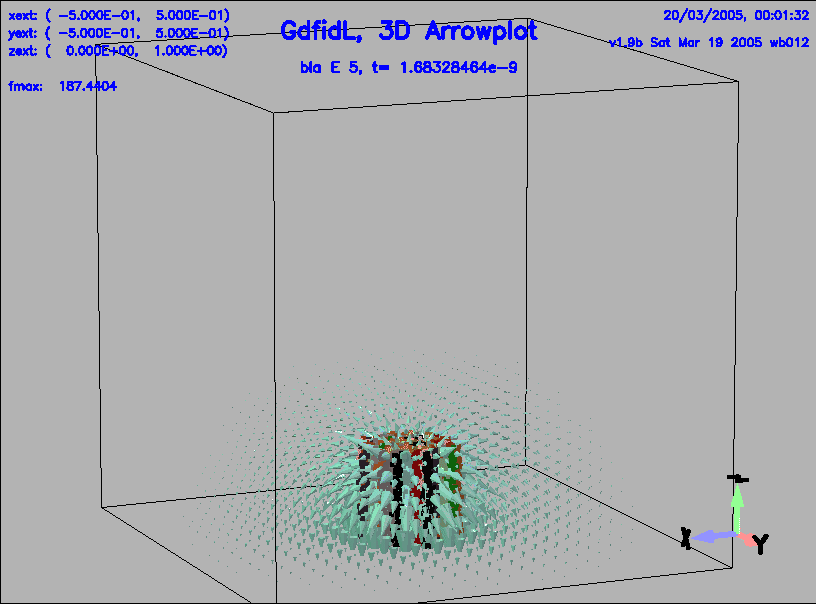
The resulting plot is shown in figure 1.
 |
The requirements read:
 Extract 1 nC of electrons from the cathode, located in the center
 of the cavity wall and having a 1 mm spot-size.
 The photoelectrons have a random distribution of longitudinal and
 transverse momentum with a total energy of 0.3 eV
 (mono-energetic for simplicity) and are extracted for 10 ps with a
 uniform time distribution (the transverse distribution is also
 uniform with cylindrical symmetry). The RF peak field on the cathode
 is 140 MV/m and the launching phase (beginning of the electron
 extraction) is 30 RF deg (90 deg is the max of the electric field).
The problem is the initial spot size of 1 mm.
To be able to resolve such a small size charged cloud, one needs a
gridspacing of 1/10 mm or less.
As the size of the phot-gun is such that it fills a volume of about
10cm x 10cm x 10cm, a gridspacing of 1/10 mm would imply a grid with
![]() cells. Although it is possible to compute with such a large number
of gridcells, we want to simulate at first with a more coarse grid,
because computing with
cells. Although it is possible to compute with such a large number
of gridcells, we want to simulate at first with a more coarse grid,
because computing with ![]() cells requires very much time and requires
some tricks.
cells requires very much time and requires
some tricks.
The inputfile for computing the resonant fields: Gun-coarse-resonant-fields.gdf We compute the resonant fields with the command
gd1 < Gun-coarse-resonant-fields.gdf | tee out-eigen
After some minutes, we get as list of frequencies:
    i   freq(i)       acc(i)         cont(i)
    1    2.8525e+9   0.0000003154  0.0000002104       # "grep" for me
    2    2.8543e+9   0.0000000211  0.0000000239       # "grep" for me
    3    4.2757e+9   0.0000000488  0.0000000718       # "grep" for me
    4    4.2757e+9   0.0000000047  0.0000006255       # "grep" for me
    5    4.2918e+9   0.0000001127  0.0000149762       # "grep" for me
    6    4.2918e+9   0.0000000907  0.0000005142       # "grep" for me
    7    4.6768e+9   0.0000000056  0.0000000338       # "grep" for me
    8    4.6768e+9   0.0000000570  0.0000001797       # "grep" for me
    9    5.4438e+9   0.0000004153  0.0000015035       # "grep" for me
   10    5.7221e+9   0.0000006921  0.0000070810       # "grep" for me
   11    5.7373e+9   0.0000355960  0.0011519827       # "grep" for me
   12    5.8261e+9   0.0017362258  0.0569873187       # "grep" for me
   13    5.8445e+9   0.0006248663  0.0431812991       # "grep" for me
   14    5.8868e+9   0.0298497210  1.0000000000       # "grep" for me
There are two resonant fields with almost the same
frequency of 2.85 GHz. Both are linear combinations of a 0-mode
and a ![]() -mode.
-mode.
We look at the two first fields:
 # Input for gd1.pp
 -gen, inf @last
 -3da, bbyhigh 0, sy e_1, do
 sy e_2, do
The resulting plots are shown in figures 2 and 3. Instead of adjusting the geometry until a pure
Inspecting the z-component of the two resonant fields:
 # Input for gd1.pp
 -gen, inf @last
 -lineplot
    sy e_1, do
    sy e_2, do
The resulting plots are shown in figures 4 and 5.
The Ez components of the two fields at the bottom of the cavity and in the center of the second cavity are
 Ez(1,1)=  842, Ez(1,2)= 840
 Ez(2,1)= -849, Ez(2,2)= 427
The requirement on the accelerating field is, the peak value of the accelerating gradient near z=0 shall be 140 MV/m. The linearcombination of the two modes, which is a pi-mode, and which has a gradient of 140 MV/m at z=0, can be found from the solution of the linear equation:
 a1 * Ez(1,1) + a2 * Ez(2,1) = 140e6
 a1 * Ez(2,1) + a2 * Ez(2,2) = 140e6
 define(INFILE, /tmp/UserName/gun-eigen )

 #
 # Load the geometry from a previously computed case:
 #
 -lgeometry
    infile= INFILE
    doit
The requirement on the accelerating field is, the peak value of the accelerating gradient near z=0 shall be 140 MV/m. The linearcombination of the two modes, which is a pi-mode, and which has a gradient of 140 MV/m at z=0, can be found from the solution of a linear equation. We can solve this system with GdfidL. In our inputfile, we solve for the amplitudes and specify that the resonant fields shall be loaded with that computed amplitudes:
 define(G0, 140e6) # Wanted Gradient

 define(v11,  842) # Gradient of first field at z=0
 define(v12,  840) # Gradient of first field at z=p/2
 define(v21, -849) # Gradient of second field at z=0
 define(v22,  427) # Gradient of second field at z=p/2

 #
 # Solve the linear system.
 #
 define(a2, (G0-v12/v11*(-G0)) / (v22-v12/v11*v21) )
 define(a1, ( -G0 - v21*a2 ) / v11 )

 #
 # Load the initial field from a previously computed case
 # INFILE is a variable, which holds the name of the resultfile
 # of the resonant field computation.
 #
 -linitialfields
    infile= INFILE, symbol= e_1, static= no, factor= a1, doit
    infile= INFILE, symbol= e_2, static= no, factor= a2, doit
The full inputfile for performing the PIC computation: Gun-coarse-pic.gdf The sourcecode for the program describing the initial conditions for the particles is Eject-beam.f90 We start the computation with the command
gd1 < Gun-coarse-pic.gdf | tee out-pic
The computation takes only some minutes.
We then start the postprocessor:
 # Input for gd1.pp
 -general, infile= @last
 ls
we get a list of datasets in the resultfile:
 bla_h_1                Hds-3D time dependent t=   33.3769e-12
 bla_e_2                Eds-3D time dependent t=   66.7538e-12
 bla_h_2                Hds-3D time dependent t=   66.7538e-12
 bla_e_3                Eds-3D time dependent t=  100.1306e-12
 bla_h_3                Hds-3D time dependent t=  100.1306e-12
 bla_e_4                Eds-3D time dependent t=  133.5075e-12
 bla_h_4                Hds-3D time dependent t=  133.5075e-12
 bla_e_5                Eds-3D time dependent t=  166.8844e-12
 bla_h_5                Hds-3D time dependent t=  166.8844e-12
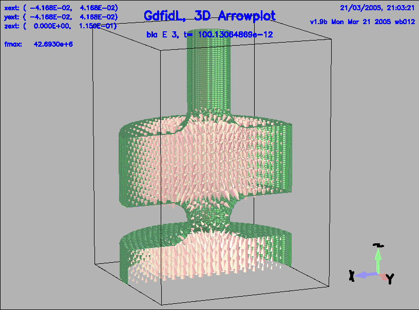
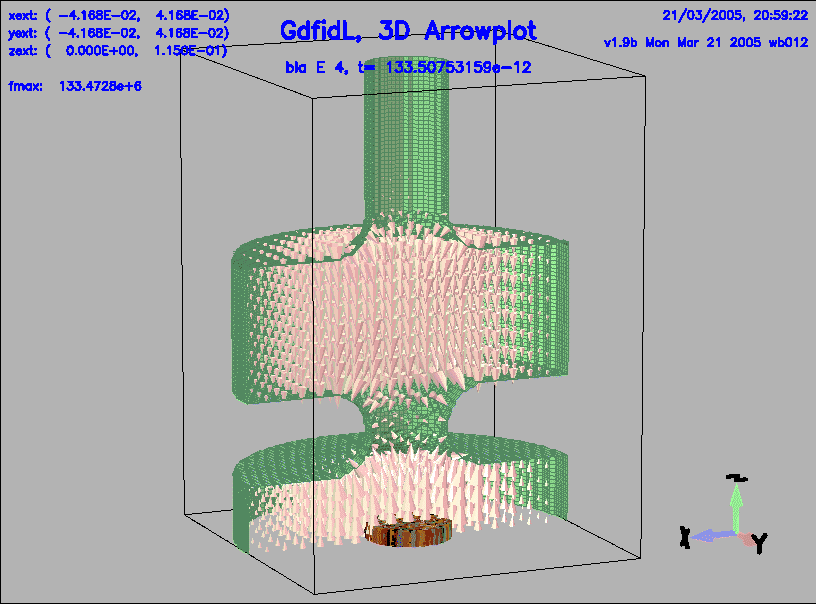
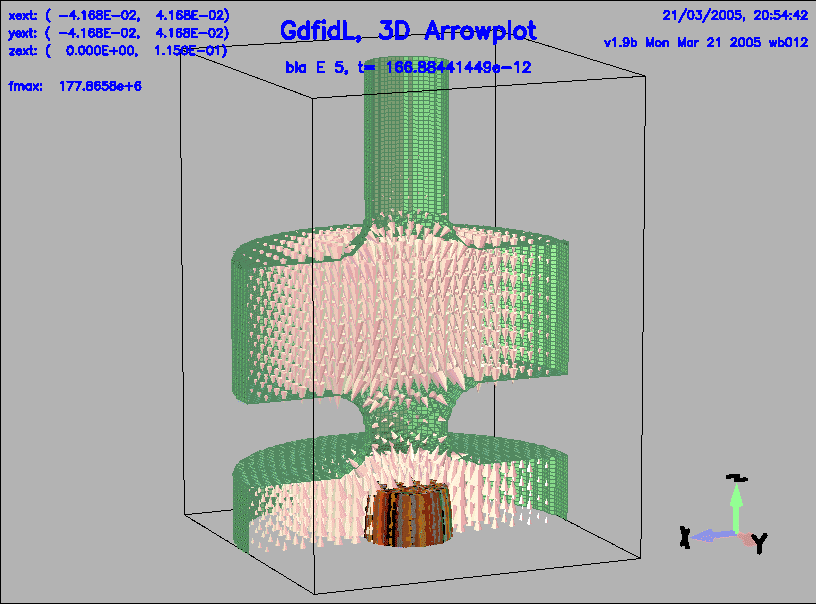
We have a look at the third, fourth and fifth stored electric field:
 -3da, bbyhigh 0
   sy bla_e_3, do
   so 4, do
   so 5, do
The resulting plots are shown in figures 6, 7, 8.
 |
 |
 |