Kazi: Longitudinal and transverse Impedances of circular symmetric Structures.

Figure 1: Lines of constant r*BPhi.
\begin{figure}\centerline{ \psfig{figure=KaziPlot.PS,width=16cm,bbllx=84pt,bblly=193pt,bburx=712pt,bbury=391pt,clip=} }\end{figure}

Figure 2: GdfidL Mesh of a Quarter of the Device.
\begin{figure}\centerline{ \psfig{figure=2Jumps.PS,width=16cm,bbllx=6pt,bblly=198pt,bburx=565pt,bbury=612pt,clip=} }\end{figure}

This Writeup publishes the Program which came out of my Diploma Thesis. This was back in 1993. The Program is written in Fortran-77, with DOUBLE COMPLEX Extension. In Fortran-77, as then Fortran-90 Compilers were just emerging. The Program solves the resulting banded linear Systems using some self developed Out-Of-Core Solver, as back then, in 1993, 64 MBytes of RAM was what a High-End Workstation would have.

The Sourcecode for the Mode Matching Program Kazi. The Sourcecode for the Program which creates Fieldplots for m=0 Plot. The Sourcecode for the Program which re-formats the Results ReFormat.

A Shell-Script which generates some Inputfile etc and creates a Plot of Fieldlines is plot.x. The resulting Plot is shown in Figure 1.

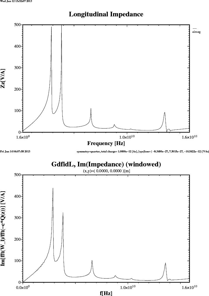
A Shell-Script which generates some Inputfile, compiles the Program, and runs the Program for computing the longitudinal Impedance (m=0), is a.x. The Results are shown in Figures 3 .. 4. The Inputfile used to compute the longitudinal Impedance with GdfidL is 2Jumps-Wz.gdf.

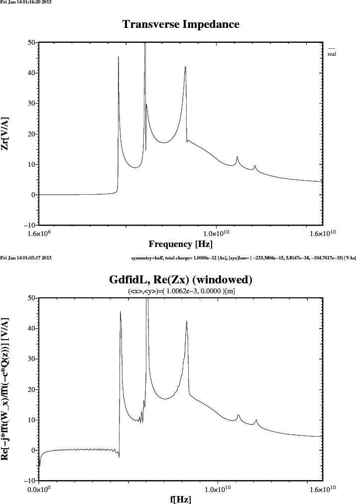
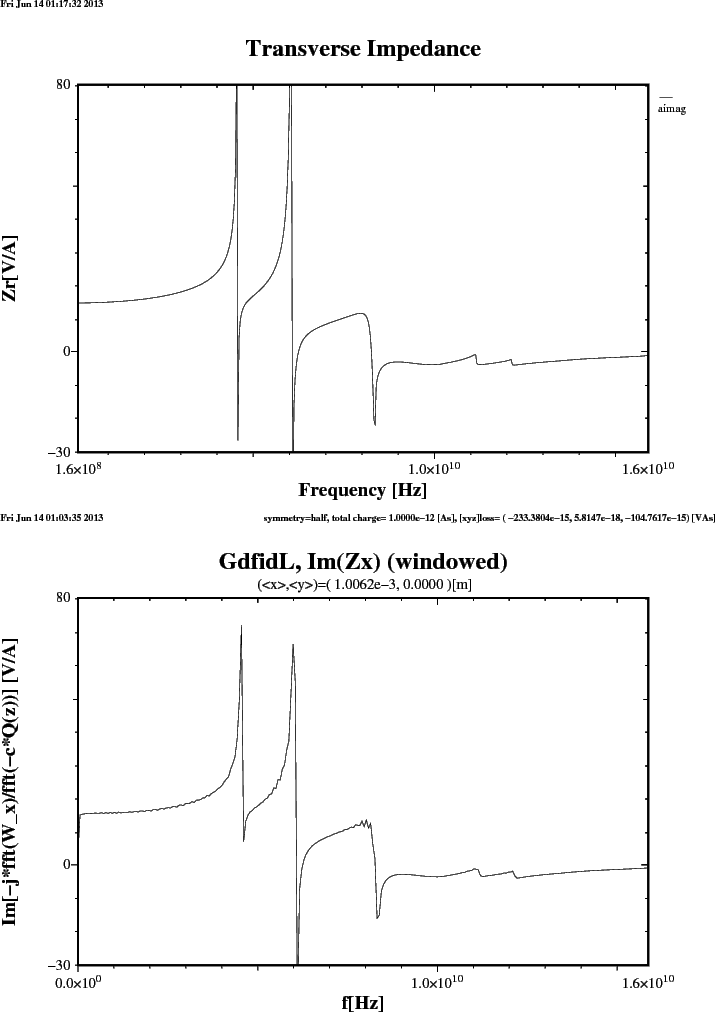
A Shell-Script for computing the transverse Impedance (m=1), is ar.x. The Results are shown in Figures 5 .. 6.

The Inputfile used to compute the transverse Impedance with GdfidL is 2Jumps-Wx.gdf.
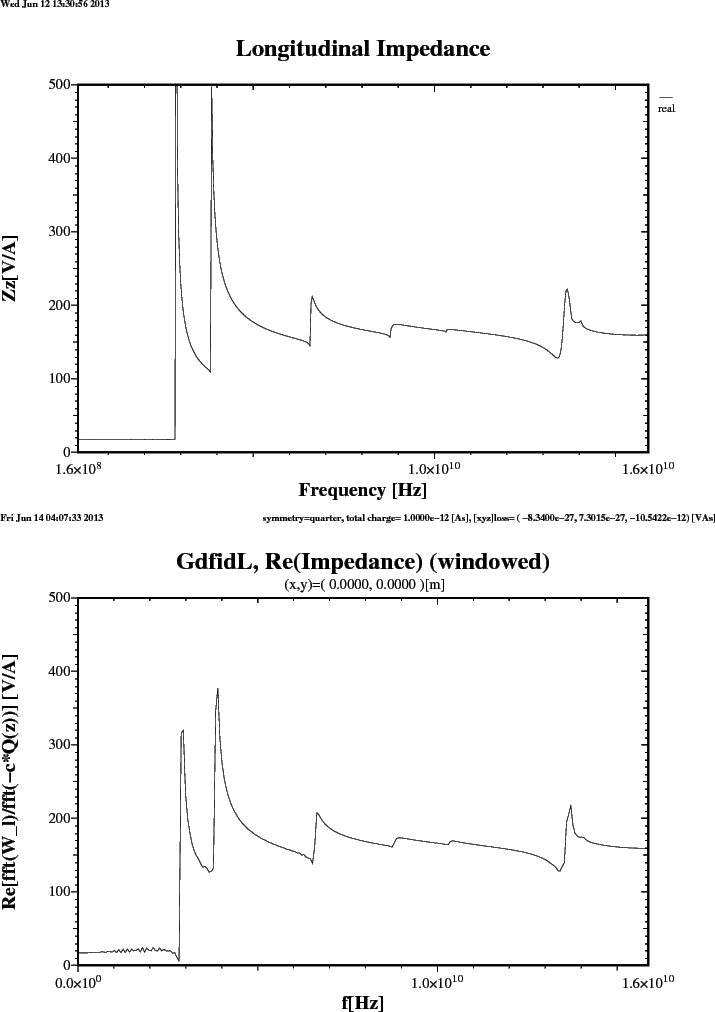
Figure 3: Top: Real Part of the longitudinal Impedance as computed by the Mode-Matching Code. Bottom: Real Part of the longitudinal Impedance as computed by GdfidL.
\begin{figure}\centerline{ \psfig{figure=RealZ.PS,width=16cm,bbllx=22pt,bblly=46...
...,width=16cm,bbllx=22pt,bblly=46pt,bburx=774pt,bbury=577pt,clip=} }\end{figure}
Figure 4: Top: Imaginary Part of the longitudinal Impedance as computed by the Mode-Matching Code. Bottom: Imaginary Part of the longitudinal Impedance as computed by GdfidL.
\begin{figure}\centerline{ \psfig{figure=ImagZ.PS,width=16cm,bbllx=22pt,bblly=46...
...,width=16cm,bbllx=22pt,bblly=46pt,bburx=774pt,bbury=577pt,clip=} }\end{figure}

Figure 5: Top: Real Part of the transverse Impedance as computed by the Mode-Matching Code. Bottom: Real Part of the transverse Impedance as computed by GdfidL.
\begin{figure}\centerline{ \psfig{figure=RealZx.PS,width=16cm,bbllx=22pt,bblly=4...
...,width=16cm,bbllx=22pt,bblly=46pt,bburx=774pt,bbury=577pt,clip=} }\end{figure}
Figure 6: Top: Imaginary Part of the transverse Impedance as computed by the Mode-Matching Code. Bottom: Imaginary Part of the transverse Impedance as computed by GdfidL.
\begin{figure}\centerline{ \psfig{figure=ImagZx.PS,width=16cm,bbllx=22pt,bblly=4...
...,width=16cm,bbllx=22pt,bblly=46pt,bburx=774pt,bbury=577pt,clip=} }\end{figure}