How to compute the External Q of a heavily loaded Cavity

Dr Alexei Blednykh of BNL had send us the Description of a Cavity where some heavily loaded Resonance near 2.7 GHz can be identified from the longitudinal Shunt-Impedance computed via a Wakepotential Computation. He could not find that Resonance in the Results of a lossy Eigenvalue Computation. This Writeup tells the Story how to find that Resonance.

The inputfile for this cavity is STL_NSLS2_LanCav.gdf

Wakepotential, Impedance

We compute with an Inputfile that is used for Wakepotential Computation, for a Time Domain Computation and for a Eigenvalue Computation with absorbing Boundaries. What is computed is selected via Parameters on the Command Line. The first Step is the Computation with a relativistic Line Charge, ie. a Wake-Potential Computation.

   gd1 -DEIGEN=0 -DWAKE=1 < STL_NSLS2_LanCav.gdf | tee Logfile

When that time-Domain Computation has sufficiently Data generated, the Postprocessor is started to compute the Impedance.

 # Input for gd1.pp
 -general, infile @last
 -wakes, impedance= yes, doit

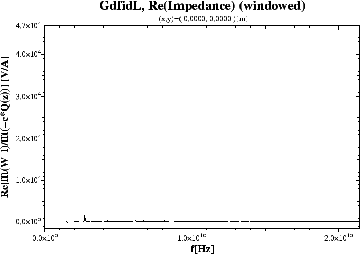
A Plot of the Real-Part of the longitudinal Impedance is shown in Figure 1. When the Region around 2.7 GHz is selected via a Mouse-Zoom, we get a Plot as shown in Figure 2. Clearly, there is a Resonance near 2.72 GHz, which is excited by the Beam and couples to the Beam.

**Figure 1:** The Real-Part of the longitudinal Impedance.
$\begin{figure}\centerline{ \psfig{figure=ReZ.PS,width=16cm,bbllx=21pt,bblly=47pt,bburx=708pt,bbury=534pt,clip=} }\end{figure}$

**Figure 2:** A Zoom of the Real-Part of the longitudinal Impedance around 2.7 GHz.
$\begin{figure}\centerline{ \psfig{figure=ReZ1.PS,width=16cm,bbllx=21pt,bblly=47pt,bburx=708pt,bbury=534pt,clip=} }\end{figure}$

Time Domain with an excited Port

To inspect what the Field of the Resonance looks like we perform a Time Domain Computation with an excited Port and store the Fields at selected Times. The excitation is such that Fields that couple to the Beam are excited, and the Excitation is such that mostly Fields near 2.72 GHz are excited.

   gd1 -DEIGEN=0 -DWAKE=0 < STL_NSLS2_LanCav.gdf | tee Logfile

When that time-Domain Computation is finished, the Postprocessor is started to generate a Plot of the Amplitude of the reflected Field, and Plots of the Field when the Excitation has sufficiently died.

 # Input for gd1.pp
 -general, infile @last
 -sparameter, time= yes, doit
 -3darrow, fonmat= yes, symbol= e_100, doit
 -lineplot, component= z, direction= z, startpoint= ( 0, 0, -99999), doit

**Figure 3:** The Amplitude of the reflected Field in time-Domain.
$\begin{figure}\centerline{ \psfig{figure=tBeamLow.PS,width=16cm,bbllx=21pt,bblly=47pt,bburx=708pt,bbury=534pt,clip=} }\end{figure}$

**Figure 4:** A Plot of the electric Field just after the Excitation has decayed.
$\begin{figure}\centerline{ \psfig{figure=tE3d100.PS,width=16cm,bbllx=0pt,bblly=0pt,bburx=708pt,bbury=534pt,clip=} }\end{figure}$

**Figure 5:** A Plot of the z-Component of the electric Field just after the Excitation has decayed.
$\begin{figure}\centerline{ \psfig{figure=tEz100.PS,width=16cm,bbllx=21pt,bblly=47pt,bburx=708pt,bbury=534pt,clip=} }\end{figure}$

Lossy Eigenvalues with absorbing Boundary Conditions

We perform an Eigenvalue Computation with absorbing Boundary Conditions.

 gd1 -DEIGEN=1 -DWAKE=0 < STL_NSLS2_LanCav.gdf | tee Logfile-Eigen

The wanted Mode is the 30.th found one. The List of Modes near the End of the Logfile:

    i            freq(i)              Q(i)       acc(i)   cont(i)
    1 ( 1.44541E+09, 1.10831E+08)     6.5208     0.00129  0.02753       # "grep" for me
    2 ( 1.47965E+09,-5.46135E+04)   -13.5465e+3  0.00375  0.08152       # "grep" for me
    3 ( 1.50022E+09,-2.43382E+04)   -30.8203e+3  0.00347  0.05900       # "grep" for me
    4 ( 1.54421E+09, 6.31150E+07)    12.2333     0.00170  0.01434       # "grep" for me
    5 ( 1.63500E+09, 4.25028E+08)     1.9234     0.00118  0.01064       # "grep" for me
    6 ( 1.65830E+09, 3.72862E+07)    22.2374     0.00135  0.04824       # "grep" for me
    7 ( 1.67591E+09, 1.08831E+08)     7.6996     0.00051  0.00730       # "grep" for me
    8 ( 1.73391E+09, 2.54403E+08)     3.4078     0.00041  0.00614       # "grep" for me
    9 ( 1.77068E+09, 3.20738E+07)    27.6033     0.00131  0.02232       # "grep" for me
   10 ( 1.82235E+09, 8.45565E+07)    10.7759     0.00064  0.01134       # "grep" for me
   11 ( 1.86006E+09, 1.18182E+07)    78.6949     0.00124  0.03053       # "grep" for me
   12 ( 1.86251E+09, 7.82413E+06)   119.0233     0.00059  0.07655       # "grep" for me
   13 ( 1.86973E+09, 4.34833E+07)    21.4994     0.00209  0.03727       # "grep" for me
   14 ( 1.92237E+09, 2.11857E+08)     4.5370     0.00028  0.00511       # "grep" for me
   15 ( 1.93942E+09, 3.56834E+09)     0.2717     0.09077  1.00000       # "grep" for me
   16 ( 1.99001E+09, 1.53246E+08)     6.4928     0.00033  0.00287       # "grep" for me
   17 ( 2.10265E+09,-5.16131E+09)    -0.2036     0.22622  1.00000       # "grep" for me
   18 ( 2.10352E+09,-1.13109E+09)    -0.9298     0.03993  1.00000       # "grep" for me
   19 ( 2.10833E+09, 2.11985E+10)    49.7282e-3  0.21832  1.00000       # "grep" for me
   20 ( 2.10950E+09, 1.39295E+08)     7.5720     0.00014  0.00235       # "grep" for me
   21 ( 2.17047E+09, 2.44018E+08)     4.4474     0.00165  0.02942       # "grep" for me
   22 ( 2.18231E+09, 1.46024E+08)     7.4724     0.00026  0.02438       # "grep" for me
   23 ( 2.19282E+09, 3.64095E+08)     3.0113     0.00056  0.01029       # "grep" for me
   24 ( 2.25231E+09, 8.71464E+07)    12.9226     0.00006  0.00073       # "grep" for me
   25 ( 2.33719E+09, 4.82227E+07)    24.2333     0.00011  0.00147       # "grep" for me
   26 ( 2.34101E+09, 2.66026E+07)    43.9996     0.00003  0.00019       # "grep" for me
   27 ( 2.50534E+09, 1.10756E+06)     1.1310e+3  0.00102  0.00772       # "grep" for me
   28 ( 2.52241E+09, 1.41953E+06)   888.4680     0.00103  0.00979       # "grep" for me
   29 ( 2.65616E+09, 1.36073E+07)    97.6004     0.00153  0.01528       # "grep" for me
   30 ( 2.72007E+09, 1.76612E+07)    77.0068     0.00048  0.00842       # "grep" for me
   31 ( 2.79701E+09, 2.66525E+06)   524.7172     0.00035  0.00643       # "grep" for me
   32 ( 2.82197E+09, 2.38525E+06)   591.5471     0.00029  0.00174       # "grep" for me
   33 ( 3.05557E+09, 1.96806E+07)    77.6291     0.00090  0.00590       # "grep" for me
   34 ( 3.13359E+09, 1.69010E+07)    92.7041     0.00076  0.00531       # "grep" for me
   35 ( 3.35784E+09, 3.02190E+08)     5.5558     0.02022  0.15663       # "grep" for me
   36 ( 3.56794E+09, 1.16206E+08)    15.3518     0.00141  0.01191       # "grep" for me
   37 ( 3.56965E+09, 1.24587E+08)    14.3259     0.00114  0.03394       # "grep" for me
   38 ( 3.62960E+09, 3.21259E+07)    56.4901     0.00157  0.04758       # "grep" for me
   39 ( 3.63499E+09, 2.73574E+04)    66.4352e+3  0.00941  1.00000       # "grep" for me
   40 ( 3.63535E+09, 1.23630E+04)   147.0248e+3  0.00456  1.00000       # "grep" for me

 # Input for gd1.pp
 -general, infile @last
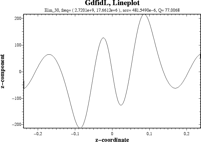
 -3darrow, fonmat= yes, symbol= ere_30, doit, symbol= eim_30, doit
 -lineplot, symbol= eim_30, component= z, direction= z, startpoint= ( 0, 0, -99999), doit

**Figure 6:** A Plot of the real Part of the electric Field of the Resonance at 2.72 GHz.
$\begin{figure}\centerline{ \psfig{figure=ere3d30.PS,width=16cm,bbllx=0pt,bblly=0pt,bburx=708pt,bbury=534pt,clip=} }\end{figure}$

**Figure 7:** A Plot of the imaginary Part of the electric Field of the Resonance at 2.72 GHz.
$\begin{figure}\centerline{ \psfig{figure=eim3d30.PS,width=16cm,bbllx=0pt,bblly=0pt,bburx=708pt,bbury=534pt,clip=} }\end{figure}$

**Figure 8:** A Plot of the z-Component of the imaginary Part of the electric Field of the Resonance at 2.72 GHz.
$\begin{figure}\centerline{ \psfig{figure=eimz30.PS,width=16cm,bbllx=21pt,bblly=47pt,bburx=708pt,bbury=534pt,clip=} }\end{figure}$