 |
The computation of the external Q of a cavity with an attached waveguide is via three simple steps.
In the first step, we compute the resonant fields in a closed geometry, ie. the waveguide is closed with an electric or magnetic boundary condition.
gd1 < cavity-with-waveguide.gdf | tee out-eigen
After some minutes we get a list of frequencies like:
  One solution seems to be static and is not saved.
    i   freq(i)       acc(i)         cont(i)
    1   27.6778e+6   0.9982920236  0.3328254536       # "grep" for me
    2    2.8818e+9   0.0000000790  0.0000000695       # "grep" for me
    3    3.6905e+9   0.0000000162  0.0000000313       # "grep" for me
    4    4.5837e+9   0.0000000003  0.0000000005       # "grep" for me
    5    6.1361e+9   0.0000000103  0.0000000206       # "grep" for me
    6    6.4118e+9   0.0000000013  0.0000000151       # "grep" for me
    7    6.6111e+9   0.0000000084  0.0000000998       # "grep" for me
    8    6.8857e+9   0.0000000062  0.0000000463       # "grep" for me
    9    7.3426e+9   0.0000000095  0.0000000774       # "grep" for me
   10    7.5733e+9   0.0000005696  0.0000093463       # "grep" for me
   11    7.6269e+9   0.0000000112  0.0000001527       # "grep" for me
   12    7.9060e+9   0.0000000082  0.0000000684       # "grep" for me
   13    8.3725e+9   0.0013724901  0.0123083161       # "grep" for me
   14    8.4666e+9   0.0060409112  0.2701361389       # "grep" for me
The inputfile for this cavity is
cavity-with-waveguide.gdf
gd1 < let-it-ring.gdf | tee out-fdtd
The inputfile for this time-domain computation is
let-it-ring.gdf
We start the postprocessor, gd1.pp, and use him interactively:
Input for gd1.pp:
     -general, infile= @last

     -sparameter
        freqdata= no
        timedata= yes
        tsumpower= yes
        doit
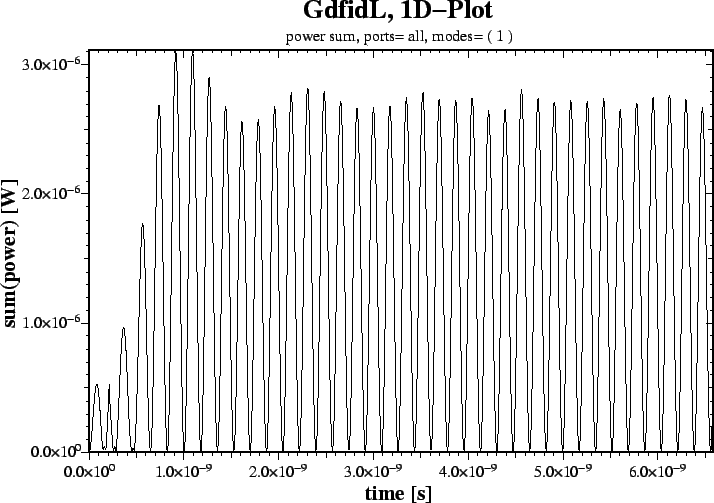
We get a lot of plots. One of these plots shows us the power sum of all
selected modes as a function of time.
..But only one mode is selected..
After about 20 periods, the transients have decayed sufficiently, leaving
only a
In order to know the external Q, we have to know what the stored energy is. Since the power flowing is almost constant, the stored energy will also be almost constant...
We compute the stored energy in the electric and magnetic field with the section "-energy" of gd1.pp:
    -energy
       solution= 8
       quantity= e, doit
       quantity= h, doit
     menu
We get the menu with 'menu'
 ##############################################################################
 # Flags: nomenu, prompt, message,                                            #
 ##############################################################################
 # section: -energy                                                           #
 ##############################################################################
 # symbol   = h_8                                                             #
 # quantity = h                                                               #
 # solution = 8                                                               #
 #                                                                            #
 #                                                                            #
 # @henergy : 4.88692e-12               (symbol: h_8, m: 1)                   #
 # @eenergy : 253.6925e-15              (symbol: e_8, m: 1)                   #
 ##############################################################################
 # doit, ?, return, end, help                                                 #
 ##############################################################################
We see that at the time when the 8.th field was stored ( t=6.6901e-9 s ), the total stored energy in the computational volume was
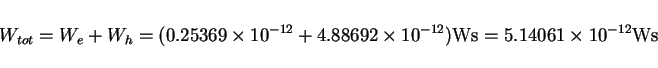 |
(1) |
The external Q for the chosen aperture width therefore is
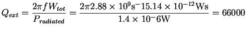 |
(2) |
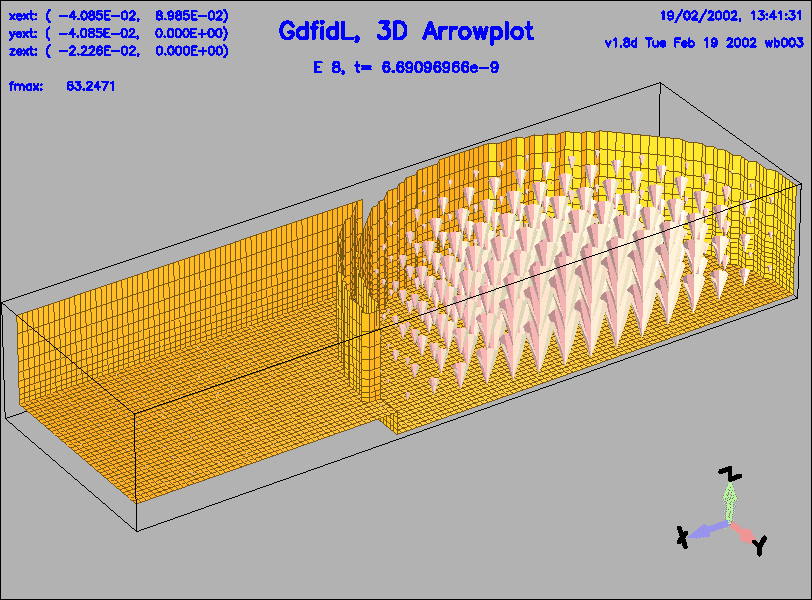
 -------
 Thats it.
Although not necessary, we want to have a look at the electric field after about 20 periods: