How to compute Cutoff-Frequencies

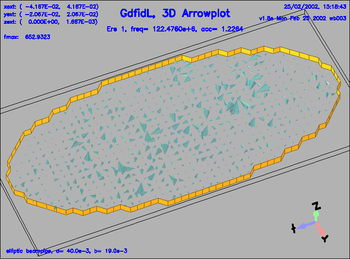
There are at least two ways to compute cutoff-frequencies with GdfidL. The easiest way is to compute resonant fields in a short section of the waveguide. When the proper boundary conditions are applied, the resulting fields and frequencies are the resonant fields at cutoff and their cutoff-frequencies.

Computation of resonant fields

The fields at cutoff can be found as resonant fields in a short section of the waveguide. Since the fields are at cutoff, they do not vary in the direction of the waveguide. The boundary conditions therefore are electric walls for TM-modes, magnetic walls for TE-modes, or periodic boundary conditions with phase shift zero for both kinds of modes.

The easiest is just to apply periodic boundary conditions with a phase shift of zero, although this is not the most computational efficient. While we are at waisting CPU-cycles, we do not even consider symmetries in the geometry of the waveguide. The computation of the cutoff-frequencies in an elliptical waveguide then is:

    gd1 < waveguide.gdf | tee out

After some seconds we get a list of frequencies like:

    i   freq(i)       acc(i)         cont(i)
    1  122.4760e+6   1.2263639315  0.4112620337       # "grep" for me
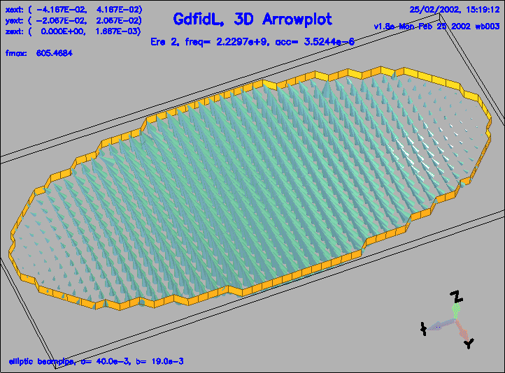
    2    2.2297e+9   0.0000035244  0.0000021997       # "grep" for me
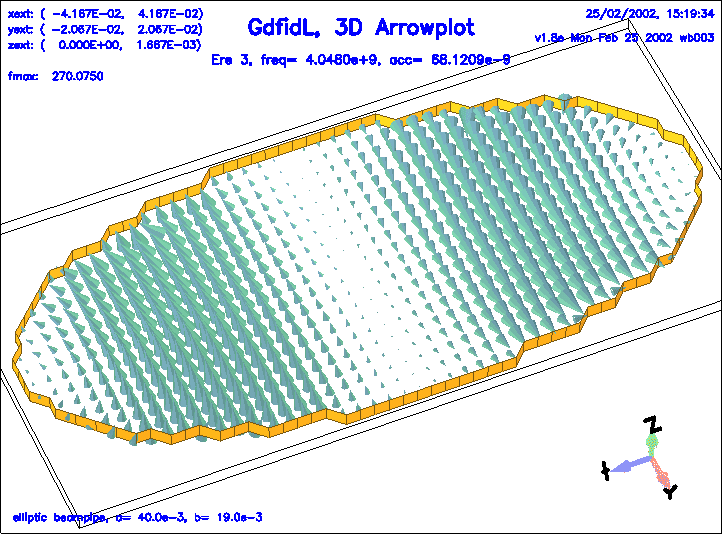
    3    4.0480e+9   0.0000000681  0.0000000812       # "grep" for me
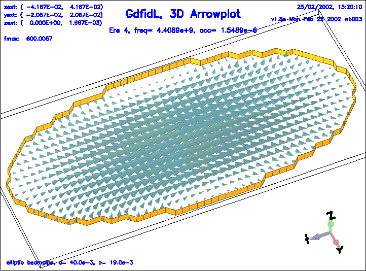
    4    4.4089e+9   0.0000015489  0.0000098211       # "grep" for me
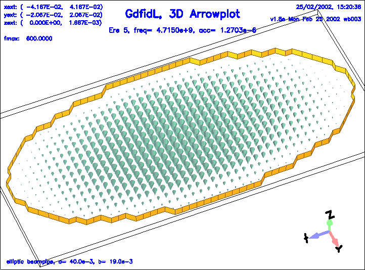
    5    4.7150e+9   0.0000012703  0.0000029069       # "grep" for me
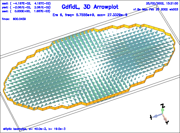
    6    5.7555e+9   0.0000000273  0.0000000753       # "grep" for me
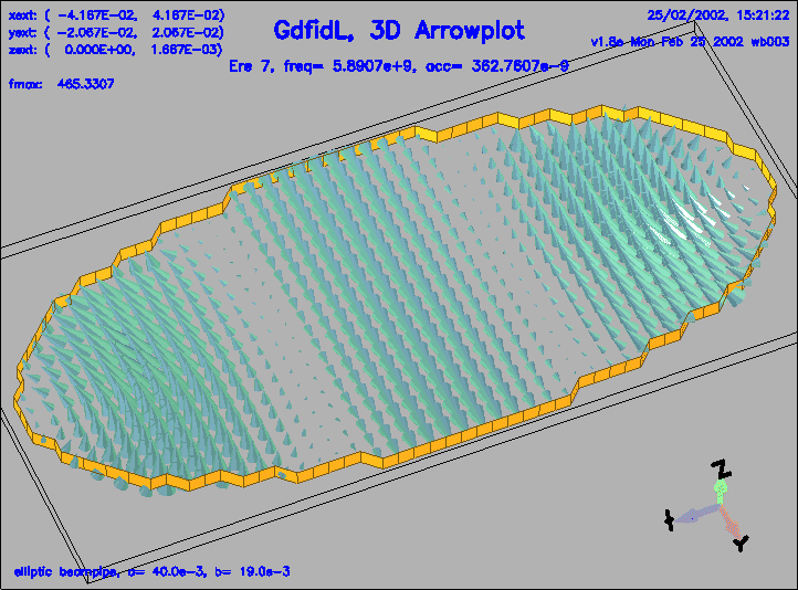
    7    5.8907e+9   0.0000003628  0.0000035260       # "grep" for me
    8    6.1920e+9   0.0000000138  0.0000000484       # "grep" for me
    9    7.0729e+9   0.0000002350  0.0000009870       # "grep" for me
   10    7.6704e+9   0.0000000257  0.0000001639       # "grep" for me
   11    7.7208e+9   0.0000001496  0.0000008549       # "grep" for me
   12    8.4049e+9   0.0000000052  0.0000000316       # "grep" for me
   13    8.5090e+9   0.0000000066  0.0000002716       # "grep" for me
   14    8.5653e+9   0.0000000160  0.0000000900       # "grep" for me
   15    9.3371e+9   0.0000000107  0.0000000643       # "grep" for me
   16    9.3944e+9   0.0000000482  0.0000005784       # "grep" for me
   17    9.7872e+9   0.0000000188  0.0000002359       # "grep" for me
   18    9.9837e+9   0.0000000028  0.0000000718       # "grep" for me
   19   10.0480e+9   0.0000000123  0.0000000657       # "grep" for me
   20   11.0034e+9   0.0000000107  0.0000000613       # "grep" for me
   21   11.0735e+9   0.0000000032  0.0000002290       # "grep" for me
   22   11.1497e+9   0.0000000023  0.0000000642       # "grep" for me
   23   11.3516e+9   0.0000000020  0.0000000512       # "grep" for me
   24   11.5672e+9   0.0000000006  0.0000000049       # "grep" for me
   25   12.2768e+9   0.0000000036  0.0000000307       # "grep" for me
   26   12.4153e+9   0.0000000038  0.0000001697       # "grep" for me
   27   12.4677e+9   0.0000000004  0.0000000200       # "grep" for me
   28   12.5967e+9   0.0000000024  0.0000001197       # "grep" for me
   29   12.6975e+9   0.0000000010  0.0000000626       # "grep" for me
   30   12.7606e+9   0.0000000009  0.0000000088       # "grep" for me
   31   13.3912e+9   0.0000000012  0.0000000132       # "grep" for me
   32   13.6535e+9   0.0000000003  0.0000000085       # "grep" for me
   33   13.8491e+9   0.0000000030  0.0000001071       # "grep" for me
   34   13.9047e+9   0.0000000011  0.0000000236       # "grep" for me
   35   14.2239e+9   0.0000000031  0.0000000697       # "grep" for me
   36   14.4204e+9   0.0000000076  0.0000002782       # "grep" for me
   37   14.5021e+9   0.0000000142  0.0000004646       # "grep" for me
   38   14.7227e+9   0.0000000058  0.0000001524       # "grep" for me
   39   15.0025e+9   0.0000000064  0.0000001735       # "grep" for me
   40   15.1974e+9   0.0000000197  0.0000007736       # "grep" for me
   41   15.3650e+9   0.0000000651  0.0000015631       # "grep" for me
   42   15.6836e+9   0.0000005207  0.0000117680       # "grep" for me
   43   16.0273e+9   0.0046087858  0.1073045033       # "grep" for me
   44   16.0768e+9   0.0039905447  0.6498775793       # "grep" for me
   45   16.1235e+9   0.0047293597  0.3225176260       # "grep" for me
   46   16.2417e+9   0.0027525493  0.0795671401       # "grep" for me
   47   16.5221e+9   0.0069169406  0.2046412339       # "grep" for me
   48   16.6937e+9   0.0606064395  0.9964082399       # "grep" for me
   49   17.2006e+9   0.0274154940  0.4583279318       # "grep" for me

The inputfile for this cavity is waveguide.gdf

Looking at the results

We use the postprocessor to look at the electric or magnetic fields at cutoff.

We start the postprocessor, gd1.pp, and use him interactively:
Input for gd1.pp:

     -general, infile= @last

     -3darrow
        fcolour= 7, eyeposition= ( 1, 2.3, 3 ), scale= 5
        quantity= ere
        solution= 2
        doit

 -------
 Thats it.

**Figure 1:** The real part of the electric field of the first computed eigenfield. This field obviously is garbage. This could also be seen from the very bad accuracy ( 1.2 ).
$\begin{figure}\centerline{ \psfig{figure=e-plot1.PS,width=16cm,bbllx=0pt,bblly=0pt,bburx=696pt,bbury=516pt,clip=} }\end{figure}$

**Figure 2:** The real part of the electric field of the second computed eigenfield. This is a TE field, and could have been found with magnetic walls at the z-borderplanes.
$\begin{figure}\centerline{ \psfig{figure=e-plot2.PS,width=16cm,bbllx=0pt,bblly=0pt,bburx=696pt,bbury=516pt,clip=} }\end{figure}$

**Figure 3:** The real part of the electric field of the third computed eigenfield. This is a TE field, and could have been found with magnetic walls at the z-borderplanes.
$\begin{figure}\centerline{ \psfig{figure=e-plot3.PS,width=16cm,bbllx=0pt,bblly=0pt,bburx=696pt,bbury=516pt,clip=} }\end{figure}$

**Figure 4:** The real part of the electric field of the fourth computed eigenfield. This is a TE field, and could have been found with magnetic walls at the z-borderplanes.
$\begin{figure}\centerline{ \psfig{figure=e-plot4.PS,width=16cm,bbllx=0pt,bblly=0pt,bburx=696pt,bbury=516pt,clip=} }\end{figure}$

**Figure 5:** The real part of the electric field of the fifth computed eigenfield. This is a TM field, and could have been found with electric walls at the z-borderplanes.
$\begin{figure}\centerline{ \psfig{figure=e-plot5.PS,width=16cm,bbllx=0pt,bblly=0pt,bburx=696pt,bbury=516pt,clip=} }\end{figure}$

**Figure 6:** The real part of the electric field of the sixth computed eigenfield. This is a TE field, and could have been found with magnetic walls at the z-borderplanes.
$\begin{figure}\centerline{ \psfig{figure=e-plot6.PS,width=16cm,bbllx=0pt,bblly=0pt,bburx=696pt,bbury=516pt,clip=} }\end{figure}$

**Figure 7:** The real part of the electric field of the seventh computed eigenfield. This is a TE field, and could have been found with magnetic walls at the z-borderplanes.
$\begin{figure}\centerline{ \psfig{figure=e-plot7.PS,width=16cm,bbllx=0pt,bblly=0pt,bburx=696pt,bbury=516pt,clip=} }\end{figure}$

Computation of resonant fields
Looking at the results